CHAPTER 02
Where the time goes
Can a slower generation step produce more tokens per second? In chapter 1, each simulated round cost one time unit. A real batch does not have a fixed price: more requests mean more computation and more data to read. Yet some work can serve several requests together. We will follow DeepInfer’s scheduled work into its operation estimate, then trace how its benchmark turns observed step returns into a reported token rate.
The question
If we put four times as many requests in a batch, how much longer can the step take before throughput falls? Which delay would an individual reader notice?
Run the next experiment and compare batches of 16 and 64:
python3 labs/05_cost.py
The script calculates costs from hypothetical rates; it does not time Python or a device. For now, each request produces one useful output token per step. Here are selected rows from its sweep:
Hypothetical model; times in microseconds
R=N  transfer  compute     step   tokens/s
  1      41.0      2.0     61.0      16393
  4      44.0      8.0     64.0      62500
  8      48.0     16.0     68.0     117647
 16      56.0     32.0     76.0     210526
 32      72.0     64.0     92.0     347826
 40      80.0     80.0    100.0     400000
 64     104.0    128.0    148.0     432432
128     168.0    256.0    276.0     463768
A batch of 16 takes 76 microseconds; a batch of 64 takes 148. Four times as many tokens cost less than twice as much time, so the aggregate output rate rises from about 211,000 to 432,000 tokens per second. But a request that stays in the larger batch waits 148 microseconds between steps instead of 76. Higher throughput and a longer token interval can occur together. The answer to the opening question is therefore: when useful output grows fourfold, throughput does not fall provided step time grows by at most fourfold.
These are two questions about the same work. Throughput counts useful output across requests per unit time. Latency measures how long a particular event takes for a request. We need a cost model to explain the first result, then a timeline to decide which latency we mean.
2.1 Give each cost a unit
Imagine a step that reads a shared array once and also reads some saved state for each request. The shared array could contain model parameters: values reused when predicting for different users. We assign four million shared bytes, another 100,000 context bytes per request and two million arithmetic operations per evaluated position. The model gives the device separate limits for memory transfer and arithmetic, plus a fixed cost that runs before either.
The constants and the complete cost function are small enough to inspect:
SHARED_BYTES = 4_000_000
BYTES_PER_REQUEST = 100_000
OPS_PER_POSITION = 2_000_000
BANDWIDTH = 100_000_000_000 # bytes/s; hypothetical
COMPUTE_RATE = 1_000_000_000_000 # operations/s; hypothetical
OVERHEAD = 20e-6 # seconds; serial in this model
def cost(requests, positions, context_scale=1, compute_rate=COMPUTE_RATE):
traffic = SHARED_BYTES + requests * BYTES_PER_REQUEST * context_scale
operations = positions * OPS_PER_POSITION
memory_s = traffic / BANDWIDTH
compute_s = operations / compute_rate
step_s = OVERHEAD + max(memory_s, compute_s)
return memory_s, compute_s, step_s
Let count active requests and count positions evaluated in this step. The transferred bytes and operation count are
Ordinary decode evaluates one position per request, so . Verification can evaluate several positions for each request: 16 requests with six positions each give , . Those positions use the same saved context. We assume that each request’s context is read once and reused across its positions, while arithmetic grows with . This isolates the benefit of reuse; traffic for new positions and intermediate arrays, repeated reads inside kernels and changes in work with context length require a richer model.
Dividing an amount of work by a rate gives a time. With memory bandwidth bytes per second and arithmetic rate operations per second,
For , transferring 5.6 million bytes takes 56 microseconds at the assigned rate. Performing 32 million operations takes 32 microseconds. A microsecond is seconds; a millisecond is seconds. Keeping seconds inside the function makes the final division into tokens per second straightforward.
If computation and memory transfer overlap perfectly, their combined duration is the larger of these two times. The script also assigns a separate serial overhead microseconds, so its step model is
| (2.1) |
The max explains the 76-microsecond result:
. The
smaller cost has not disappeared. Under this overlap assumption, it finishes before the larger
one.
2.1.1 A bound is not a stopwatch
If and are upper limits on achievable rates, then is a lower bound for the time needed to move those bytes and perform those operations. It becomes the script’s predicted duration only because we assume perfect overlap and attainment of both rates. Adding also assumes that this overhead cannot overlap with either activity.
Actual work can violate those scheduling assumptions. Some operations depend on data that has not arrived; small device programs, called kernels, may not reach the assigned rates; several stages may each have a different bottleneck. Conversely, host work counted in may overlap with device work. Do not add the maximum of two whole-step totals and expect it to describe every dependency inside the step. Chapter 6 will give those dependencies their own timeline.
The model tells us which assumption to investigate. An arithmetic optimisation can leave a transfer-limited step unchanged because arithmetic does not determine its duration.
2.2 Find what batching shares
First keep , as in the opening sweep. At small , the four-million-byte shared read dominates the memory cost. More requests spread that read, and the fixed overhead, across more useful outputs. At larger , the arithmetic cost catches up. The crossover occurs where , with both times in microseconds: . Figure 2.1 plots both costs and the resulting output rate.
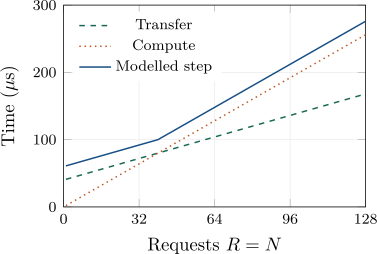
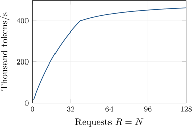
labs/05_cost.py. Both panels use
ordinary decode, with one evaluated position and one useful token per request per step
().
The left shows the competing costs; the right shows output throughput. Both plots read
the CSV saved by the experiment.
For , equation 2.1 becomes microseconds. The output rate is therefore
It approaches 500,000 tokens per second as the fixed cost becomes a smaller fraction of each step. Latency keeps growing. There is no single best batch size until we also state a latency limit, memory capacity and available work.
This reasoning is the basis of the roofline model: arithmetic throughput is bounded by the smaller of compute capacity and bandwidth times arithmetic intensity, , measured in operations per byte. The original paper calls this operational intensity and counts traffic between cache and main memory [18]. Here the crossover has operations per byte: 80 million operations divided by eight million bytes. The roofline bound excludes our separately added serial overhead ; our plots show step time and token rate, rather than a conventional roofline plot.
This saving relies on the shared read actually being shared. A mixture of experts (MoE) model routes positions to selected parameter arrays called experts. A larger batch can touch more experts, so the shared-byte term need not stay fixed. Chapter 7 will follow this cost across devices in Wide-EP. Similarly, a batch of longer contexts can require more saved-state traffic per request. The next two lines change one condition at a time:
One change at a time (microseconds)
R=N=16, double compute rate: 76.0 -> 76.0
R=N=32, four times context traffic: 92.0 -> 188.0
Doubling the arithmetic rate at reduces its compute term from 32 to 16 microseconds. Transfer still takes 56, so the step remains 76. Multiplying the per-request traffic by four at raises the transfer term from 72 to 168 microseconds, and the step grows from 92 to 188. The argument for batching survives; the cost curve changes with the workload.
2.2.1 More positions can reuse the same context
Now hold the request count at 16 and increase only the evaluated positions. The experiment keeps transfer at 56 microseconds:
Same 16 requests, more positions (microseconds)
 R   N  transfer  compute     step
16  16      56.0     32.0     76.0
16  28      56.0     56.0     76.0
16  96      56.0    192.0    212.0
At , compute catches up with transfer, yet the step still takes 76 microseconds. The extra 12 positions add no step time under our assumptions. At , compute takes 192 microseconds and the step takes 212. Reusing context makes some verification work cheap; it does not make unlimited work free. Nor are evaluated positions necessarily useful output tokens.
2.2.2 Bytes per element are part of the model
An array’s element count does not yet tell us its byte count. A conventional 32-bit value occupies four bytes; a 16-bit value occupies two. Lower-precision formats can use fewer bits for values while storing extra information needed to interpret groups of them. Allocation alignment can add further padding.
For example, an invented format holding 32 one-byte values plus one two-byte scale occupies 34 bytes, or 1.0625 bytes per value. Multiplying the element count by one would miss the scale. The example illustrates accounting, not a particular DeepInfer layout.
The deployment Q&A gives a concrete unit for later chapters: 528 bytes per token per stored layer for its MXFP8 sliding-window attention KV state [2]. That is a layout size, not a whole-model per-token budget. We will count layers and retained positions when we derive memory requirements. For a traffic estimate, we must also establish how often those bytes are read. Bytes retained in memory and bytes transferred during a step are different quantities.
2.3 Count useful output separately
In the ordinary-decode sweep, evaluated positions produce useful tokens. Verification breaks this equality. A later chapter will let a cheaper predictor propose tokens that the main model checks; some checked positions may not become output. Let be the useful output from a step. The rate we want is
| (2.2) |
For repeated steps of different sizes, measure total useful tokens divided by total elapsed time. Averaging individual step rates without weighting their durations answers a different question.
The cost script finishes with two assigned useful-output counts for the same 16 requests, evaluating either 32 or 64 positions:
Assigned useful-output counts; rate = U / step_s
R=16, N=32, U=24: 84 us, 285714 useful tokens/s
R=16, N=64, U=28: 148 us, 189189 useful tokens/s
The second choice produces more useful tokens per step, 28 instead of 24, but its time grows from 84 to 148 microseconds. Both choices read the same context; the additional arithmetic causes the increase. The useful rate falls. These assigned counts are an arithmetic exercise; chapter 8 will derive expected output from acceptance probabilities. Its policy will need both that numerator and a cost curve for the denominator.
This distinction already matters in DeepInfer. The deployment Q&A describes DSpark allocating verification work using predicted acceptance and a profiled hardware throughput curve. Its table estimates a change from fixed-5 to variable-length verification of at 16 concurrent requests per rank, but at 96 [2]. Our model suggests a reason for this trend: at low concurrency, removing positions may save little time because transfer still dominates; as concurrency grows, reducing verification arithmetic can shorten a compute-limited step. This is an interpretation, not a reproduction of those figures. Chapter 8 will combine acceptance with measured costs; the hypothetical constants cannot choose a production budget.
2.4 Read a request timeline
A step duration does not say how long a user waits for the first token. The next experiment reads
labs/data/06_request_trace.json, a saved teaching trace with assigned timestamps. All
events use the same observation clock and all times are in milliseconds. The records specify
arrival, the start and end of prompt processing, and the delivery time of every output
token.
python3 labs/06_trace.py
Before running it, consider request E. It arrives at 3, starts prompt processing at 30, ends that span at 42, and delivers tokens at 45, 49 and 65. How much of its first-token wait occurs before prompt work starts? Figure 2.2 marks the boundaries the script uses.

For arrival , prompt start , prompt end and token delivery times , the script computes
Time to first token (TTFT) includes queueing in this definition. The time between tokens is a sequence of gaps , rather than one number. We call the publish gap in this book; DeepInfer does not use that name. It covers everything between the recorded end of prompt processing and the first delivery, and need not be one operation.
These boundaries are chosen for the experiment. In a service, arrival might mean receipt by a gateway, admission to an engine or transmission from a client. Token delivery might mean an engine callback or data reaching the client. Those choices include different queueing, transfer and buffering costs. Write them down before comparing two measurements. Real records from several clocks also need clock alignment before we can subtract their timestamps.
Here is the complete calculation for one request:
def analyse(request):
arrival, start, end = (request[key] for key in ("arrival", "prompt_start", "prompt_end"))
tokens = request["tokens"]
assert tokens and arrival <= start <= end <= tokens[0]
assert tokens == sorted(tokens)
queue, prompt, publish = start - arrival, end - start, tokens[0] - end
ttft = tokens[0] - arrival
gaps = [later - earlier for earlier, later in zip(tokens, tokens[1:])]
assert ttft == queue + prompt + publish
return queue, prompt, publish, ttft, gaps
The saved output includes all five requests:
Synthetic teaching trace: assigned timestamps, not engine measurements
All times in ms; gaps exclude the wait for the first token
id  queue  prompt  publish  TTFT  gaps
A       2       6        2    10  4,4,4
B       2       6        2    10  -
C       8       8        3    19  4,4
D       8       4        3    15  4
E      27      12        3    42  4,16
TTFT: n=5, mean=19.2, p50=15, p95=42
Token gaps: n=8, mean=5.5, p95=16
Whole trace: 13 tokens / 65 ms = 200.0 tokens/s
E waits 27 milliseconds before prompt processing begins, then spends 12 in the prompt span and three in the publish gap. Its TTFT is 42 milliseconds. Its later gaps are four and 16 milliseconds. Shortening the first-token queue would not, by itself, remove that last pause. Conversely, reporting only its later token gaps would hide the long initial wait.
A faster kernel can leave first-token latency almost unchanged when the request spends most of its time waiting to run. Suppose an illustrative request waits 30 milliseconds, then takes 10 milliseconds to reach its first token. Halving all of that latter work reduces TTFT from 40 to 35 milliseconds, not to 20. The timeline tells us which part an optimisation can shorten.
The prompt span measures elapsed time between two markers, not pure arithmetic. If a real request’s prompt work is chunked and interleaved with other requests, that span can include intervening waits. Likewise, device execution, host processing and delivery can overlap across requests. Adding every recorded operation duration is not generally a way to recover wall-clock time.
2.4.1 Look beyond an average
The five TTFTs have a mean of 19.2 milliseconds, but the slowest request waits 42. The script also reports sample percentiles. It sorts the values and chooses the element at rank , counting ranks from one:
def percentile(values, fraction):
"""Nearest-rank percentile of a non-empty sample, for 0 < fraction <= 1."""
return sorted(values)[ceil(fraction * len(values)) - 1]
The sample median, or p50, is 15 milliseconds. With only five values, p95 is the maximum, 42. This tiny example shows the calculation; it cannot estimate a production tail reliably. Real comparisons need enough requests, a workload description and a stated percentile convention.
There are eight later-token gaps, with mean 5.5 milliseconds and p95 of 16. Request B has only one output token, so it contributes no gap. Substituting zero would invent an observation. Pooling all gaps also weights requests with more output tokens more heavily than requests with fewer; averaging one mean per request is another convention.
Finally, the script counts 13 output tokens over the 65 milliseconds from the first arrival to the last delivery: 200 tokens per second. This whole-trace rate includes the initial waits and final completion. It is not a steady-state decode rate. An observation window chosen to include only busy steps would have a different denominator.
2.5 Trace work and measurements through DeepInfer
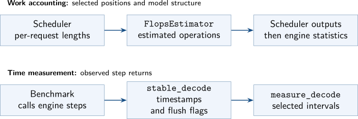
Chapter 1 followed requests through admission, scheduling and execution. We now follow the quantities attached to that work: selected positions, estimated operations, observed intervals and reported throughput. Figure 2.3 adds two paths around the same engine. Keeping them separate prevents a common mistake: treating a count of operations as if it were a measurement of the time taken to execute them.
2.5.1 From scheduled positions to an operation count
The C++ scheduler constructs per-request metadata after selecting a batch. Inside its loop over selected sequences, it obtains two lengths:
int seqlen_q = scheduler_outputs.seqlens_q[i];
int seqlen_k = seq->cache.num_tokens + seq->schedule.total_inflight_tokens + seqlen_q;
Here seqlen_q counts the new positions selected for this request. seqlen_k
extends the cached prefix by pending positions and the new work. For an assigned
example with 128 cached positions, two in flight and three selected, the metadata has
,
. It
does not say that all 133 positions have completed. The pending term connects directly to the
delayed worker state from chapter 1.
Across requests, the sum of selected values plays the role of in our cost model; the number of selected requests plays the role of . Two batches with the same can have different request counts and context lengths. The teaching model represents that difference with context bytes per request. DeepInfer retains individual lengths and model structure rather than reducing every step to one batch-size scalar.
When statistics are enabled, the same metadata-construction loop calls an estimator and adds its two results to the batch totals:
if (log_stats) {
const bool is_prompt = scheduler_outputs.prompt_run;
const int full_len = seq->input.tokens.get_len();
const auto [attn, total] =
flops_estimator->calc_flops(seqlen_q, seqlen_k, is_prompt, full_len, is_prompt ? seq->cache.swa_valid_start : 0);
attn_flops += attn;
total_flops += total;
}
The call’s extra arguments describe prompt extent and which sliding-window state is valid. Chapters 3 and 9 will explain why these boundaries affect the model’s work. For now, follow the returned pair into the estimator itself:
// Return (attention, total); total already includes attention. Scheduler
// calls this directly from its existing per-request metadata construction.
std::pair<int64_t, int64_t> calc_flops(int q, int k, bool is_prompt, int full_len, int swa_valid_start = 0) const {
const auto [full, consumer] = query_ranges(q, k, is_prompt, full_len, swa_valid_start);
const int64_t attn = calc_attn_flops(full, consumer, is_prompt);
const int64_t non_attn = calc_non_attn_flops(full.rows(), consumer.rows());
const int64_t logits = calc_logits_flops(q, is_prompt);
return {attn, attn + non_attn + logits};
}
The method derives row ranges, counts attention, counts other model operations and counts the projection that produces token scores, called logits. Its return value is , not three independent counters. Adding its two returned numbers would count attention twice. The two row ranges accommodate differences between layers; chapter 9 explains the full and consumer row ranges when it counts truncated prefill.
Back in the scheduler, lines 730–731 divide the accumulated counts by
and
store them in attn_tflops and total_tflops. Despite their names, these fields hold
tera-operation amounts for the scheduled batch, not operations per second. The engine copies
them into StepStats during post-processing. No elapsed time appears in the estimator call or
that unit conversion [8, 14, 5].
Notice the direction of the dependency: selected lengths feed this logging branch. This call is not choosing the verification budget. DSpark’s documented use of a profiled cost curve is a different path, which chapter 8 will trace. The distinction matters when locating code to investigate a scheduling choice.
2.5.2 An operation estimate has a scope
A floating-point operation is often abbreviated to FLOP. Counting a multiply and an addition as two operations is a common convention. DeepInfer’s estimator goes further: it assigns format-dependent weights to express work in FP8-equivalent FLOPs.
// GEMM coefficients include multiply-add (2 FLOPs) and the FP8-equivalent weight.
namespace flops_coef {
constexpr int64_t FP4 = 1;
constexpr int64_t FP8 = 2;
constexpr int64_t BF16 = 4;
constexpr int64_t TF32 = 8;
constexpr int64_t FP32 = TF32; // Accounting reference, not actual kernel precision.
} // namespace flops_coef
// Estimate main-model work in FP8-equivalent FLOPs; FP32/TF32 use weight 4.
// Count major contractions regardless of bottleneck; exclude draft/padding/replicas.
// MFU measures target-model FLOPs throughput; DFlash is extra compute used
// to accelerate that model, so its FLOPs are excluded.
// Omit small arithmetic (norms/activations). TODO: vision.
// Scheduled q/k ignore acceptance/ZOS corrections.
The comments use GEMM for matrix multiplication and MFU for model FLOPs utilisation, which compares the model’s arithmetic rate with a compute-capacity reference.
FP8 denotes an eight-bit floating-point format family; FP4 uses four-bit values, and BF16 is a sixteen-bit format. The coefficients here describe normalised arithmetic accounting, not bytes per element. The factor for a multiply-add is already included: the FP8 coefficient is two and the BF16 coefficient is four. The comment’s FP32/TF32 precision weight of four likewise becomes the code’s coefficient of eight after multiplication by two. Dividing this estimate by an arbitrary device’s advertised operation rate would mix conventions unless the rate uses compatible weights and scope [14].
The comments also exclude draft-model work, padding and replicas, and say that scheduled lengths have not incorporated acceptance or ZOS corrections. The and values we traced are therefore scheduling-time inputs to an accounting estimate, not a complete record of what every kernel finally ran. A higher main-model FLOPs rate does not prove that a request completed sooner, especially if extra work outside that count was used to obtain it.
2.5.3 A benchmark chooses its observation window
Now follow the lower path in Figure 2.3. The benchmark drives the same LLMEngine.step that
chapter 1 inspected, but it controls when step returns enter a measurement window. A bounded
queue stores timestamps and flags:
stable_prefill: deque[tuple[int, float, bool]] = deque(maxlen=prefill_measure_steps + 1)
stable_decode: deque[tuple[float, bool]] = deque(maxlen=decode_measure_steps + 1)
decode_measure_steps is 60 in this edition, so the decode queue holds 61 endpoints.
Adjacent endpoints define 60 intervals. This is a different use of a queue from the scheduler’s
waiting: it stores observations, not requests available to run.
The surrounding control flow separates unmeasured work from collection:
for _ in range(decode_warmup_steps):
if not llm.llm_engine.has_unfinished_requests():
break
run_decode_step(measure=False)
set_engine_log_interval(20)
for _ in range(decode_measure_steps):
if not llm.llm_engine.has_unfinished_requests():
break
run_decode_step(measure=False)
set_engine_log_interval(0)
while len(stable_decode) < stable_decode.maxlen and llm.llm_engine.has_unfinished_requests():
run_decode_step(measure=True)
The first loop performs up to 50 warm-up steps. The next performs up to 60 unmeasured steps
with a different logging interval. Only the final loop calls run_decode_step(measure=True).
Filling 61 entries can require more than 61 calls because the inner function also checks the
running-request count. Every loop can stop early when no unfinished requests remain. A separate
profiler segment follows this window; its calls use measure=False.
The benchmark records a host timestamp after step() returns, and only when the
running-request count matches its requested decode concurrency:
def run_decode_step(*, measure: bool) -> None:
countdown_before = lb_flush_countdown() if measure else None
llm.llm_engine.step()
if measure and len(llm.llm_engine.scheduler.running) == args.decode_num_requests:
flushed = countdown_before is not None and lb_flush_countdown() > countdown_before
stable_decode.append((time.perf_counter(), flushed))
flushed here tracks expert-load-balancing statistics flushes. It does not mean the final
in-flight-request flush from chapter 1. The interval calculation filters out steps marked by those
statistics flushes:
clean = [ts - prev[0] for prev, (ts, flushed) in pairwise(stable_decode) if not flushed]
if not clean:
return {}
avg_sps = len(clean) / sum(clean)
The numerator is the number of selected intervals; the denominator is their summed
duration. The timestamps are qualifying step-return boundaries, not per-request token
arrivals. If an intervening call fails the concurrency check, it creates no entry, but its
elapsed time can still lie between stored endpoints. There is no separate counter of those
omitted calls in stable_decode. The selected-window rate is most straightforward when
concurrency stays stable, which is what the benchmark arranges its workload to study
[15].
2.5.4 Follow one interval through the filter
Use four assigned endpoint times to read the filter. These milliseconds are illustrative inputs, not benchmark results; the implementation stores seconds.
| Endpoint (ms) | Flush flag | Interval (ms) | Treatment |
| 0 | False | — | First endpoint only |
| 4 | False | 4 | Keep |
| 10 | True | 6 | Exclude |
| 15 | False | 5 | Keep |
pairwise forms adjacent pairs before the comprehension applies its filter. The flag at
10 excludes the interval from 4 to 10; the next pair still starts at 10. The result is
, about
222.2 selected intervals per second. Removing the flagged endpoint first would incorrectly join 4 to 15,
giving ,
about 133.3. The order of pairing and filtering is part of the metric’s definition.
The source detects a statistics flush when its countdown increases across the step. This
protects the chosen comparison from that maintenance cost; it does not make the cost disappear
from service execution. If no eligible intervals remain, measure_decode returns an
empty dictionary. A caller must not interpret that as a measured zero-throughput
run.
2.5.5 From a local step rate to a reported token rate
The output dictionary converts that step rate into a token rate with this line:
"decode_tokens_per_s_per_gpu": avg_sps * args.decode_num_requests * (envs.DEEPINFER_USE_NEXTN_DECODE + 1) / cp_size,
The source itself explains how to interpret and convert this metric. Here are the complete
comments on lines 405 and 407 (author’s translations; nextn is the configured draft
length):
“With VARLEN=0, each step always submits tokens, so it is independent of acceptance rate.” (Line 405, attached to
decode_avg_sps.)“Full-acceptance accounting: count tokens per request per step; to use a different , recalculate from
decode_avg_sps.” (Line 407.)
Here is the average useful output per request per step. The fixed submission size is the premise for holding step rate fixed while changing that output count. It is not a guarantee that every other runtime cost is invariant.
For an illustrative cp_size=1, 16 requests, 200 steps per second and five draft tokens, it reports
tokens per
second. Using
at that same step rate gives useful throughput of 9,600. This is the conversion the
comment describes. With VARLEN=1, acceptance affects the number of submitted positions
and hence can change step rate, as the comment on line 539 also warns. We must
measure that policy’s time and useful output together, rather than reuse the fixed-length
timing.
The denominator cp_size also needs a scope. The launcher runs a separate request batch
for each data-parallel (DP) rank, and only rank 0 writes the metrics. Each rank uses
cp_size devices for context parallelism (CP), which shares its context work across those
devices. Thus this “per GPU” metric divides rank 0’s local request throughput by its CP
device count; it is not a sum over all ranks divided by all devices. Here ep_size is
the total device count and dp_size the number of request-serving ranks, with
. Equal
rates across ranks would make the two averages agree, but this reporting code does not check that
condition [15, 16, 17]. Preserve useful output counts and elapsed times for every rank needed in a
system-wide comparison.
measure_decode returns its dictionary to the rank-0 reporting block. That block formats the
console result and can save configuration together with the measured fields:
if args.result_jsonl is not None:
result = benchmark_config | prefill_metrics | decode_metrics
args.result_jsonl.parent.mkdir(parents=True, exist_ok=True)
with args.result_jsonl.open("a", encoding="utf-8") as f:
f.write(json.dumps(result, default=str) + "\n")
print(f"Benchmark result appended to {args.result_jsonl.resolve()}")
The saved decode fields include the selected interval count, step rate and maximum selected interval, plus the full-acceptance token rate. They do not contain the raw endpoint queue or observed useful token counts. Recomputing a rate under another assumed is possible; auditing a different interval filter or the realised useful output requires additional records. This follows from the dictionary being written, not from the file’s JSON format.
We can now locate three different changes. To change which calls count as measurement,
inspect the window loops and run_decode_step. To change the exclusion rule, inspect the
pairwise comprehension. To replace full-acceptance accounting with useful throughput, obtain
useful counts over the same time window before changing the reporting formula. Editing the
FLOPs estimator would address none of those three questions.
A cost curve belongs to a hardware setup
The deployment Q&A puts support for multiple accelerator vendors among its system goals. The inspected release supports NVIDIA SM100 and Huawei Ascend 950; its README limits batch-invariant inference to NVIDIA [1, 2].
Record the platform, numerical formats, kernels, parallel layout and measurement boundary with a curve. A result on one setup is not a rate constant for another. The model above can organise either investigation, but its parameters must come from the setup being studied.
The next chapter opens the context-byte term in this model. It explains what the cached rows contain, which reads remain after caching, and how DeepInfer’s attention layout determines their size.
2.6 Experiments to try next
- Impose a 150-microsecond step limit in the hypothetical model. Which integer request count, with , gives the highest output rate within it? What changes if per-request traffic is multiplied by four?
- Halve the fixed overhead, then halve the arithmetic cost. Compare the effects at and . Which assumption makes each change useful? Then hold and find the largest that adds no time over ordinary decode.
- In a scratch copy of the trace, delay all of E’s token deliveries by ten milliseconds without moving its prompt markers. Which of TTFT, publish gap, later-token gaps and whole-trace throughput change?
- For a benchmark report, write down the numerator, the time endpoints and any excluded intervals. Which additional raw count would let you turn a full-acceptance rate into an observed useful-output rate?
- In the assigned endpoint table, mark the endpoint at 15 as a flush too. Which interval
survives? Then mark the endpoint at 4 as a flush: which branch of
measure_decoderuns, and what should a report say? - Locate the logging branch that calls
calc_flops. Explain why reducing its estimate alone cannot change the number of positions selected for verification or the benchmark’s reported token rate.