CHAPTER 03

The model shapes the engine

Chapter 2 counted context bytes as an input to its cost model. What do those bytes contain, and why must the engine keep reading them? Chapter 1 saved a running sum whose state fitted in one number, however long the input became. Attention keeps rows of numbers, and a new query can read many of them. What does caching save if the engine still has to read the past?

Run a small attention calculation:

python3 labs/07_attention.py

The inputs are five vectors, each containing two numbers. The script first rebuilds the calculation for every growing prefix, then repeats it while keeping keys and values. Its first comparison reports:

full: cached outputs match every recomputed prefix
projected rows: recompute=15, cache=5
query/key pairs: recompute=35, cache=15
retained KV rows: 5
last output: 2.790791, 0.930264

The cached calculation projects five input rows instead of fifteen. It also avoids recalculating the outputs for old positions. But it still evaluates fifteen query/key pairs: one for the first position, two for the second, and so on up to five. Caching removes repeated work on the past; the current query still consults that past.

We will make those rows visible before opening DeepInfer’s model code. The source walk then follows one layer with sliding-window attention (SWA) from its input to a cache write and an attention read. Along the way, three different quantities will emerge: the number of visible positions, the number of allocated positions and the bytes needed to represent one position.

3.1 A query chooses a mixture

A vector is an ordered list of numbers. Its dot product with another vector of the same length multiplies corresponding entries and adds the products: $[1,2]\cdot [3,4]=1\cdot 3+2\cdot 4=11$. Attention uses such a score to decide how much one position should contribute to another.

Each input row produces a query, a key and a value. The query describes what the current position seeks. Each key supplies a score against that query. The values supply the numbers that will be mixed. Our lab uses simple fixed projections:

12def project(x):
13    a, b = x
14    return (a, b), (a - b, a + b), (a + 2 * b, 2 * a - b)

In a trained model, learned arrays determine these transformations. Here the small formulas let us inspect every entry:

position | input = query | key     | value
       0 | (1, 0)        | (1, 1)  | (1, 2)
       1 | (0, 1)        | (-1, 1) | (2, -1)
       2 | (1, 1)        | (0, 2)  | (3, 1)
       3 | (2, 0)        | (2, 2)  | (2, 4)
       4 | (0, 2)        | (-2, 2) | (4, -2)

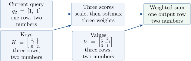
At position 2, the query is $[1,1]$. It can see keys at positions 0, 1 and 2. Their dot products are $2,0,2$. Divide each by $\sqrt{2}$, where two is the query width. This scaling is part of scaled dot-product attention [19]. We then turn the scores into positive weights that sum to one. The operation is called softmax: exponentiate each score and divide by the sum of the exponentials. A larger score gets a larger share.

For scores $s_j$, the weight of position $j$ is

Subtracting the same maximum leaves the mathematical ratios unchanged and keeps the largest exponent at zero. Each output entry is a weighted sum of the corresponding entries in the value rows:

17def attend(query, keys, values):
18    scores = [sum(a * b for a, b in zip(query, key)) / sqrt(len(query))
19              for key in keys]
20    peak = max(scores)
21    masses = [exp(score - peak) for score in scores]
22    total = sum(masses)
23    weights = [mass / total for mass in masses]
24    return tuple(
25        sum(weight * value[d] for weight, value in zip(weights, values))
26        for d in range(len(values[0])))

In Figure 3.1, one query row meets three key rows. The resulting three weights multiply three value rows, producing one output row. A matrix is simply a rectangular array of such rows. For $N$ queries of width $d$, $L$ keys of width $d$, and values of width $d_v$, the shapes are

The familiar expression $\text{softmax}(Q{K}^T∕\sqrt{d})V$ describes the same calculation for several query rows. The transpose turns each key row into a column so that matrix multiplication computes all the dot products.

3.2 Cache the past, calculate the present

Generation uses causal attention: position $i$ can see positions 0 through $i$, including itself, but no later position. A later token therefore cannot change an earlier output in this layer. With fixed model parameters and unchanged earlier inputs, the earlier keys and values remain valid when another input arrives.

The incremental loop projects one new row, appends its key and value, and calculates only the new output:

41def incremental(xs, window=None):
42    keys, values, outputs = [], [], []
43    pairs = 0
44    for x in xs:
45        query, key, value = project(x)
46        keys.append(key)
47        values.append(value)
48        if window is not None:
49            keys, values = keys[-window:], values[-window:]
50        outputs.append(attend(query, keys, values))
51        pairs += len(keys)
52    return outputs, pairs, len(keys)

With window=None, the lists grow. Old queries are not needed to calculate the new output, but old keys and values are. In a causal stack of layers, the same argument applies layer by layer: each layer keeps its own state derived from that layer’s inputs.

The lab’s recomputation baseline projects every row and calculates every causal output in each prefix. Across prefixes of lengths 1 through 5, that is $1+2+3+4+5=15$ projected rows and $1+3+6+10+15=35$ query/key pairs. The cached version projects five rows and calculates fifteen pairs. These counts compare two specified algorithms; they are not instruction counts for an optimised kernel.

The script checks every output in every prefix with absolute and relative tolerances of $10^{-12}$. The mathematical calculation is unchanged. The test permits floating-point rounding differences; it does not establish bitwise agreement between different device kernels.

For a long context of length $L$, one full-attention decode query still uses $L$ keys and $L$ values. Its score and mixture work grow with $L$, as does the amount of logical KV data it consumes. During prefill, many queries are available together, allowing kernels to reuse data across them. This is the distinction between requests $R$ and evaluated positions $N$ in chapter 2: several queries for one request can share its context. The number of logical references alone does not tell us how many bytes cross a particular memory interface.

3.2.1 Give each query a window

A sliding window of width $W$ changes the visible range to

The current position occupies one of the $W$ places. Figure 3.2 shows the resulting band of visible positions.

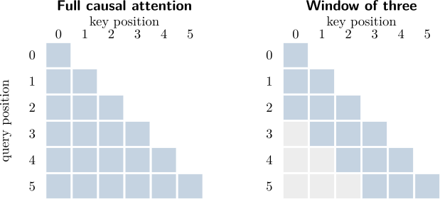
The same incremental loop implements a window by retaining only its last $W$ keys and values. For $W=3$, the experiment reports:

window=3: cached outputs match every recomputed prefix
projected rows: recompute=15, cache=5
query/key pairs: recompute=31, cache=12
retained KV rows: 3
last output: 3.000000, 1.000000

After the window fills, each new query reads three rows. Across five queries, the pair count is $1+2+3+3+3=12$. The last output is $[3,1]$, whereas full attention returned approximately $[2.790791,0.930264]$. We can check the windowed result by hand. The final query is $[0,2]$; the last three keys all have second component 2. Their dot products are therefore all 4, and their scaled scores are all $4∕\sqrt{2}$. Softmax gives each row weight $1∕3$. The corresponding values are $[3,1]$, $[2,4]$ and $[4,-2]$, whose average is exactly $[3,1]$.

These are two separate comparisons. Caching agrees with recomputation under the same visibility rule. Restricting full attention to a window changes the rule and can change the output. Whether a model performs its task well with that restriction is a model-quality question; agreement between two implementations cannot answer it.

Chapter 1’s last-three-numbers exercise recovered its state exactly from those raw inputs. This lab also projects each row directly from a fixed input. At a deeper model layer, the inputs themselves can depend on earlier attention. Replaying a short suffix need not reconstruct those inputs exactly. Chapter 9 will examine that different contract.

3.3 Count rows, then count bytes

A model usually calculates several attention mixtures, called heads, at each layer. Several query heads may share the same stored keys and values. For memory accounting, count stored KV heads rather than assuming that each query head owns a separate copy.

For an illustrative model with separate K and V arrays of equal width, let $n_{\ell }$ be the number of layers, $h_{\mathit{KV}}$ the stored KV heads, $d$ their width, $L$ the context length and $b$ the bytes per element. One request’s KV payload is

The factor two counts keys and values. A model whose every layer uses a window $W$ needs at most

for those visible rows. These formulas exclude allocation padding, other state and temporary buffers.

python3 labs/08_kv_layout.py

With 32 layers, eight KV heads, width 128, a context of 4,096 and two-byte elements, the lab gives:

generic full KV: 536,870,912 B = 512 MiB
generic window KV: 16,777,216 B = 16 MiB

One mebibyte (MiB) is $2^{20}$ bytes. A 128-position window reduces this example’s payload from 512 MiB to 16 MiB. Independent requests multiply the capacity requirement; shared prefixes and shared layers need their own ownership accounting.

The element size must describe the actual representation. BF16 uses two bytes per value. An eight-bit quantised value uses one byte, but its scale factors also need storage. Quantisation represents numbers with a smaller set of values, generally introducing error. A capacity calculation can count those bytes without claiming that the resulting model is numerically identical.

3.4 Open DeepInfer’s attention path

Before following one attention call, locate it inside the prediction function from chapter 1. A token ID first selects a learned vector, its embedding. Successive layers transform these vectors into hidden states: the current representations of the input positions. Attention mixes information across visible positions. A feed-forward sublayer transforms each position’s representation using learned weights; in a mixture of experts (MoE), a gate chooses which expert networks perform that transformation. Chapter 7 follows those experts across devices.

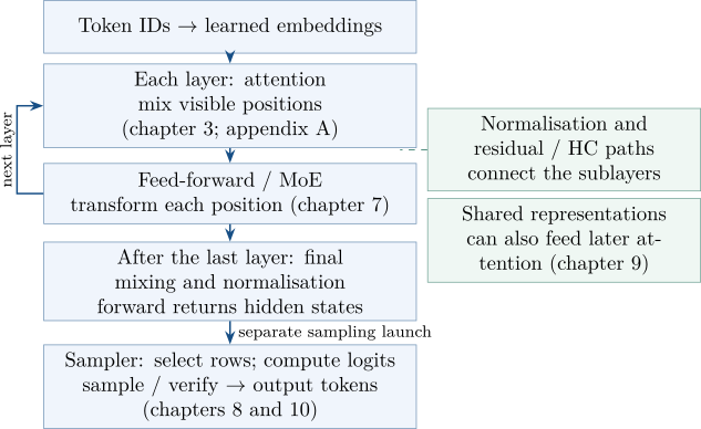
DeepInfer’s text path makes these stages concrete. In deepinfer/model_executor/models/deepseek.py, DeepseekModel.forward looks up input embeddings at lines 160–162 and calls the layers at lines 210–218. The layer’s forward in the adjacent decoder_layer.py calls self.self_attn at lines 155–161, then self.mlp at lines 169–173 [20, 21].

Normalisation and residual paths connect these transformations. A simple residual adds a sublayer’s input to its output, preserving a route for the earlier representation. DeepInfer also supports hyper-connections (HC), which mix several residual streams; the figure marks that surrounding machinery without deriving it. Appendix B locates HC and the additional Engram embedding path. Chapter 9 opens a different connection: a shared hidden representation that supplies later attention layers.

The main forward returns hidden states, not token IDs or vocabulary scores. DeepseekForCausalLM.sample passes those states and lm_head.weight to Sampler; its get_logits call produces the vocabulary scores for selected rows. Sampling then chooses output tokens or verifies drafts [20, 58]. Thus chapter 6’s separate forward and sampling launches have a real data boundary. Chapters 8 and 10 open the sampling stage. Here we follow the persistent state read by attention inside the layer stack.

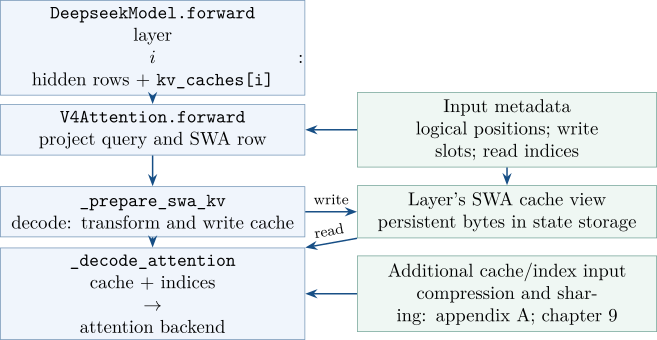
The generic two-array formula is useful, but it is not DeepInfer’s cache layout. The V4 path stores a shared KV representation, supplies explicit indices to its attention backend, and may combine SWA with another cache. We will follow the SWA part of an ordinary decode step. Compression, sparse selection and cross-layer sharing remain named inputs here; Appendix A follows them into the attention read. Figure 3.4 marks the path we take through the layer.

3.4.1 Project the current rows

DeepseekModel.forward passes each layer its hidden states and its cache view; the decoder layer forwards these to V4Attention, along with position and address metadata [20, 21]. The cache survives the call. Of the model loop’s optional inputs, cross_layer_runtime carries cross-layer state, embed_hook supplies an n-gram embedding lookup, and dflash_input holds input for the draft model.

Inside V4Attention.forward, projection and cache preparation are adjacent:

787q_a, kv_swa = self._project_q_and_swa(
788    hidden_states,
789    shared_hidden_bf16,
790)
791del hidden_states, hidden_states_bf16, shared_hidden_bf16
792kv_swa, wait_kv_swa = self._prepare_swa_kv(
793    kv_swa,
794    kv_cache.swa_cache,
795    input_metadata,
796    use_cp,
797)
798
799q_b, index_q_b = self._project_q_b(q_a, input_metadata.positions)
800del q_a

For a layer without shared-hidden input, _project_q_and_swa applies one combined projection and splits its output into q_a and kv_swa. The former is an intermediate query representation; _project_q_b expands it into query heads. With $N$ evaluated positions, $H$ query heads and width $d$, the resulting query layout is $N\times H\times d$. The new SWA projection has $N\times d$ elements, with one shared row per position rather than a separate stored row for each query head [22].

This is already an architectural constraint on the engine. It must keep the projected representation expected by this model and backend, rather than allocate separate K and V arrays for every stored head. The projection and normalisation details need not be mastered to follow the lifetime of that storage.

3.4.2 A decode projection writes persistent state

In the decode branch of _prepare_swa_kv, the output destination is a cache plus a write-slot mapping:

422assert not use_cp
423cast_args = CastArgs(
424    "e4m3",
425    self.swa_cache_num_per_channels,
426    round_sf=True,
427    sf_format="ue8m0",
428)
429out_args = KVCacheOutArgs(
430    swa_cache,
431    input_metadata.slot_mapping_store_swa,
432)

cast_args selects the smaller numerical format. out_args pairs the cache with the assigned write slots. The fused operation receives both alongside the parameters for transforming the row:

433result = fused_norm_rope_hadamard_cast_store_kvcache(
434    kv_swa,
435    norm_args=NormArgs(self.kv_swa_norm.weight, self.kv_swa_norm.variance_epsilon),
436    rope_args=RopeArgs(
437        input_metadata.positions,
438        self.rotary_emb.cos_sin_cache,
439        self.qk_rope_head_dim,
440        self.rotary_emb.is_neox_style,
441        offset=self.qk_head_dim - self.qk_rope_head_dim,
442    ),
443    cast_args=cast_args,
444    out_args=out_args,
445)
446if not input_metadata.is_prompt:
447    assert result is None
448    return None, None

Read the arguments before the long function name. norm_args supplies normalisation parameters. rope_args supplies position-dependent rotations, commonly called rotary positional embeddings or RoPE. The output arguments direct the result into swa_cache at slot_mapping_store_swa.

The assertion and return at the end matter: decode expects no returned tensor from this operation. Its useful result is the change to persistent cache storage. A reader who follows only Python return values would miss that state transition.

3.4.3 The 528-byte row is defined in code

The SWA allocation calls _kv_bytes_per_token with use_fp4=False. That helper selects V41_FORMAT and checks that the model dimensions and scale grouping match it [23]. Its definition is short:

109V41_FORMAT = KVCacheFormat(
110    quantized_dtype="e4m3",
111    quantized_elements=512,
112    elements_per_sf=32,
113    bf16_elements=0,
114    do_cast=True,
115    sf_format="ue8m0",
116    note="V41, main/swa kv.",
117    token_interleaved=True,
118)

There are 512 eight-bit values, with one scale per 32 values. ue8m0 is the encoded scale format; this implementation stores each scale in a one-byte unsigned integer. The format’s properties therefore give

This agrees with the deployment Q&A’s MXFP8 SWA figure [24, 2]. It includes scale overhead. There is no additional factor two: keys and values use the same stored row.

This is the cache-saving idea behind Multi-head Latent Attention (MLA), introduced in DeepSeek-V2. Instead of retaining expanded keys and values for every head, MLA retains a smaller learned representation, a latent vector, from which both are obtained. The query heads share that latent state. The V2 paper also caches a separate position-encoding component; its complete cache is not just the latent vector [28].

The inspected V4 implementation has its own layout. The cache helper asserts kv_lora_rank + rope_head_dim == layout.num_elements; V41_FORMAT fixes that total at 512. This combines the latent and position-related dimensions, rather than counting 512 ordinary key elements per query head. The model’s Wkv projects into this shared space. The backend, decode_mla_mqa_sparse, uses the row for key scoring and value accumulation: its call receives head_dim_v=self.qk_head_dim, with no separate value cache. The accumulated context is transformed by _wv_and_o_proj afterwards [23, 29, 22].

Compare one layer and one token in the two layouts:

The first uses about 7.76 times as many bytes. This compares the illustrative separate-K/V layout with the inspected SWA row; it includes differences in head sharing, dimensions and precision. It is not a measured compression ratio for the same model. Both quantities are per layer per token, before multiplying by window length or counting other model state.

The cache engine exposes part of its allocated state storage as a tensor view:

418assert start % 32 == 0
419if blocks is not None:
420    swa_cache = blocks[:, start : start + swa_size].as_strided(
421        (blocks.shape[0], swa_block_size, 1, swa_size_per_token), (blocks.stride(0), swa_size_per_token, swa_size_per_token, 1)
422    )

The shape is

as_strided supplies both shape and distances between entries in the underlying allocation. The leading stride is blocks.stride(0): moving to another request’s state slot can skip more than this layer’s SWA region. The one in the third dimension records the shared KV layout. The final dimension counts bytes, including scales, rather than 528 independent model features.

The second lab separates visible rows from allocated rows:

SWA row: 512 data B + 16 scale B = 528 B
128 visible rows, one layer: 67,584 B
134 allocated rows, one layer: 70,752 B

The 128-position window specifies what attention may use. We can derive the 134-position ring from the code. In cache_engine.py, lines 88–93, get_inference_swa_block_size adds DEEPINFER_MAX_BACKTRACKING_TOKENS to the window. In deepinfer/environ.py, lines 129–132, the draft limit DEEPINFER_USE_NEXTN_DECODE defaults to 5; the backtracking allowance is the larger of an explicit override (zero when unset) and that limit plus one:

The cache helper’s docstring explains the purpose: “nextn requires backtracking by n tokens” (author’s translation) [23, 30]. The expression chooses six extra positions, so this is a configured allowance rather than simply the five possible drafts.

This separates the model’s requirement from the engine’s execution choice. The window determines which positions a query may see; the draft configuration adds room for backtracking. The default 134 is their combination, not a new attention window or a constant prescribed by MLA. As with the shared latent row, the useful comparison is between what the model needs to read and what the engine must retain to execute it safely.

Decode metadata uses get_kvstore_swa_block_size. With DEEPINFER_PREFILL_STORE_EXTRA_STATE disabled, as it is by default, that helper returns the same 134. Enabling it adds DEEPINFER_PREFILL_STORE_EXTRA_SIZE, whose default is 128. Within that enabled branch, YOCO truncation (chapter 9) also adds the non-negative configured DEEPINFER_YOCO_PREFILL_KEEP_TOKENS when truncation is on. Thus the lab’s $S=134$ follows the default environment settings for a 128-token window; overrides can enlarge it. Chapter 4 follows the resulting allocations. The separately configured replay-retention length, such as 140, is not the attention window or the default ring size.

3.4.4 Trace a window boundary and a ring boundary

For a query at position $p$, let $S$ be swa_block_size and $b$ be state_id. The logical length is $\text{min}(p+1,W)$. A position $p$ occupies flattened slot

The modulo wraps within one request’s ring. Multiplying the state ID by $S$ selects that request’s block. These flattened slots count token rows; they are not byte offsets or Python object addresses.

Use the default $W=128$, $S=134$, and choose state ID $b=2$. This request owns flattened slots 268 through 401. The scalar transcription in the lab produces:

position | logical range | first/last read slot | write slot
     127 |   0..127       | 268 / 395            | 395
     128 |   1..128       | 269 / 396            | 396
     133 |   6..133       | 274 / 401            | 401
     134 |   7..134       | 275 / 268            | 268

At position 127, attention can see logical positions 0 through 127. At position 128, position 0 leaves the window and position 128 enters. The write goes to slot 396; the ring has not wrapped.

At position 134, the logical window is 7 through 134. Its physical read indices are 275 through 401, followed by 268. The write to 268 replaces logical position 0, which left the visible window six steps earlier. It does not replace the oldest visible position, 7. Window eviction and physical overwrite are different events when $S>W$.

The lab checks partial windows, repeated wraps and separation between state IDs. It implements the inspected address formulas using Python integers. It does not run the metadata kernel. The source path is what connects the calculation to DeepInfer’s arrays.

3.4.5 Expand the read indices

The CUDA decode-metadata kernel constructs those bounds and write slots:

138swa_len = T.min(pos + 1, window_size)
139window_start_pos = pos - swa_len + 1
140swa_off = state_id * swa_block_size + window_start_pos % swa_block_size
141kv_swa_index_offset_len[q_off, 0] = swa_off
142kv_swa_index_offset_len[q_off, 1] = swa_len
143
144slot_mapping_store_swa[q_off] = state_id * swa_block_size + pos % swa_block_size

V4Attention.forward calls compute_attn_info before projecting the new rows. On decode, that method calls get_kv_swa_index_decode if the index array has not yet been prepared. It obtains the physical ring length from get_kvstore_swa_block_size [25]. The index helper receives two sizes: window_size determines the number of output columns; swa_block_size determines physical wraparound. The helper selects the index kernel’s ring branch [25, 26]:

59else:
60    for j in T.Parallel(B):
61        index[j] = offset // block_size * block_size + (offset + i * B + j) % block_size
62for j in T.Parallel(B):
63    index[j] = T.if_then_else(i * B + j < length, index[j], -1)
64T.copy(index, kv_index[bx, i * B : (i + 1) * B])

Here $\mathit{iB}+j$ is an output column processed by the kernel, not a model position or a batch size. The division recovers the block base from the first read offset. The modulo wraps the successive columns inside that block. Columns beyond the valid length receive $-1$, so a short request does not read unfilled positions.

3.4.6 The attention read consumes cache and indices together

After the new SWA rows have been stored, the decode path supplies the cache and its read indices to the backend:

640if self.use_swa:
641    attn_kv_args = dict(
642        key_cache=kv_cache.swa_cache,
643        indices_in_kvcache=kv_swa_index,
644        key_cache_extra=kv_cache.ca_cache,
645        indices_in_kvcache_extra=kv_ca_index,
646        index_length_extra=dense_index_len,
647    )

The additional cache fields keep another source of context visible in the interface. They prevent a misleading conclusion: a 128-token SWA component does not mean that the whole V4 model can use only 128 tokens. This chapter’s capacity and visibility bounds apply to the SWA component.

Those arguments reach the attention operation here:

660    context, _ = decode_mla_mqa_sparse(
661        q_b,
662        head_dim_v=self.qk_head_dim,
663        sched_meta=input_metadata.flash_mla_sched_meta_dict[self.sched_meta_key],
664        softmax_scale=self.softmax_scale,
665        attn_sink=self.attn_sink_params,
666        batch_invariant=envs.DEEPINFER_BATCH_INVARIANT,
667        fused_norm_rope_cast_kwargs=fused_kwargs,
668        **attn_kv_args,
669    )
670return context

q_b supplies the current queries. The cache arguments supply stored rows, and softmax_scale is initialised to $d^{-1∕2}$, the scaling used in the lab. The returned context is then passed to _wv_and_o_proj to produce the attention sublayer’s output [22].

The backend also explains a potentially surprising detail. Its non-fused FlashMLA call sets causal=False. The comment at attention_backend.py:133 says, in the author’s translation, “sparse attention supports only non-causal mode” [27]. This call therefore asks the kernel to apply no causal mask of its own. The index rows must exclude future positions; otherwise the kernel could read them. Causality is enforced by the address construction we just traced.

3.5 Keep visible rows safe from overwrite

During decode, the current row is stored before attention reads the window. Could prefill do the same for a whole chunk? A chunk may write slots whose old contents are still needed by its early queries.

The prompt branch therefore constructs a temporary attention input. It places current SWA rows after the cached SWA rows, with any compressed rows after those. It loads the old window before storing the new one:

845if self.use_swa:
846    if input_metadata.is_prompt:
847        load_paged_kv_cache(
848            kv_cache.swa_cache,
849            input_metadata.load_segments_swa,
850            total_k_swa_cached,
851            out=kv[:total_k_swa_cached],
852        )  # [num_seqs * window_size, 1, qk_head_dim]
853        kv_swa_full_index = input_metadata.kv_swa_full_index  # [total_q, window_size]
854        # The SWA store slots may overlap the ranges loaded above, so prefill must store only after the cache load.
855        store_kv_cache(kv_swa, kv_cache.swa_cache, input_metadata.slot_mapping_store_swa)
856    else:
857        kv_swa_index = input_metadata.kv_swa_index  # [total_q, window_size]

The prefill indices refer to the assembled input, whereas decode indices refer directly to cache slots. The two branches implement compatible visibility through different physical layouts.

For a small example, take a window of three and a ring of five. Suppose the cached prefix ends at position 3 and the new chunk contains positions 4, 5 and 6. Query 4 needs old positions 2 and 3 plus new position 4. Query 6 needs only new positions 4, 5 and 6. Writing positions 5 and 6 wraps into slots 0 and 1, which are harmless in this particular chunk. Extend the chunk through position 7, however, and its write to slot 2 would destroy position 2 before query 4 had read it. Loading the old rows first makes all these queries safe to compute together.

3.5.1 Several decode queries can also overwrite old rows

The same hazard applies to a verification step. With five available draft tokens and fixed-length verification, one request supplies six query positions, $p,\dots ,p+5$. This is a decode call: the scheduler marks its output as non-prompt, and the model metadata preserves that choice. Its SWA path writes the new rows before the attention read. Chapter 8 follows the draft and verification machinery; here we use only its query count and write order [31].

For a full window, the earliest query, at $p$, needs old rows beginning at $p-127$. In a ring of length $S$, writes at $p,\dots ,p+5$ replace the previous occupants at $p-S,\dots ,p+5-S$. Avoiding damage to that earliest query requires

This is a derived lower bound for these six writes, not a proof that 133 satisfies every engine requirement. With $S=128$, the last five writes replace rows still needed by query $p$. The default $S=134$ satisfies the bound and preserves the configured backtracking allowance. The lab checks all six queries after the writes for $S=128,133,134$:

S=128: overwritten visible rows per query = [5, 4, 3, 2, 1, 0]
S=133: overwritten visible rows per query = [0, 0, 0, 0, 0, 0]
S=134: overwritten visible rows per query = [0, 0, 0, 0, 0, 0]

Each entry counts visible rows whose previous contents were overwritten for that query. The two mechanisms now have a common explanation: prefill copies old rows before overwriting them; decode reserves space beyond the visible window.

The model therefore shapes both the cache representation and its access rules. The next chapter follows the storage behind these views: who allocates a state slot, which requests may share state, and when the engine can reuse it.

3.6 Experiments to try next

1. Change the attention lab’s window to one, then to a value larger than the input length. With one, each output should equal its own value row. With the larger window, outputs should agree with full attention. Keep the prefix-agreement checks.
2. In the layout lab, change the generic KV-head count from eight to one. Explain why query-head count does not occur in its capacity function. Then halve the element size and identify which quantisation overheads the generic formula still omits.
3. Trace state ID 3 at position 134 with a 134-position ring. Derive the first read slot, last read slot and write slot. They should be 409, 402 and 402. Explain why none belongs to state ID 2.
4. In the prefill example, extend the chunk through position 8. Which other old row would an early store destroy, and which queries still need it? Use the checklist below to review the ordering.