CHAPTER 09
Reconstruct state approximately
Chapter 1 rebuilt a three-entry window by replaying three inputs. Chapter 4 then encountered state that DeepInfer deliberately leaves out of its persistent cache. Rebuilding that state sounds like the same operation. The difficulty is what an entry contains: a later layer caches representations produced by earlier layers, and those representations may depend on positions outside the window. DeepInfer shortens prefill by accepting an approximation in this local state, while preserving the full source for another part of the cache.
The question
If each layer reads only three positions, can replaying the last three inputs rebuild two layers’ caches exactly? What changes if both layers take their cached entries from the same shared input?
python3 labs/19_replay.py
The lab starts with the integers 1 to 8, two layers and a window of three. Each layer adds the mean of its visible entries to its current input. One version caches each layer’s own input; the other always caches the shared original input. It compares a full prefill with a replay of inputs 6, 7 and 8, then uses each resulting cache to process the next input, 9:
KV source    last row (full / suffix)  next row (full / suffix)
shared          22 / 22                   25 / 25
per-layer       28 / 57/2                 32 / 193/6
Shared inputs preserve both results. Per-layer inputs change the last prefill result from 28 to , and the next decode result from 32 to . The error survives the handover from prefill to decode. We will find the same dependency distinction in DeepInfer’s full block-KV projections and truncated sliding-window attention (SWA).
9.1 Where exact window recovery stops
The lab uses identity KV projections: the cached row is the input row itself, and the attention weights are uniform. For a layer input and cached values , its rule is
Here is the window and is the first available position. The full calculation starts at zero; suffix replay starts later. The addition of is a residual: it carries that row’s input into its output. This deliberately small rule isolates the dependencies without introducing softmax or floating-point round-off.
The two versions differ in one line of the layer loop. boundary is the unchanged input, while
hidden is the preceding layer’s output:
caches = []
for _ in range(depth):
kv = boundary if shared else hidden
caches.append(kv[-window:])
output = []
for i, value in enumerate(hidden):
visible = kv[max(0, i - window + 1):i + 1]
output.append(value + sum(visible) / len(visible))
hidden = output
return hidden, caches
Consider the per-layer version. The first layer’s full output at the position holding 6 is . Replaying from 6 loses 4 and 5, giving . At the positions holding 7 and 8, the replay gives and 15, instead of 13 and 15. These three outputs become the second layer’s KV rows. Its last query therefore reads different values even though all three positions are present:
The first changed cache entry is in layer 2, at zero-based position 5. Recovering the raw entries recovered layer 1’s KV, but did not recover the representations needed by layer 2.
In the shared version, both layers read the original values 6, 7 and 8 for the last position. That position’s residual is also unchanged: it had its whole window in the preceding layer. Its final result is . The retained shared KV is exact even though some earlier retained hidden rows are not. More generally, with shared KV, row-local operations and a replay that contains the last row’s window, the last row stays exact by induction over layers: its own previous representation and its visible shared KV are unchanged. This reasoning also permits queries that depend on that row’s previous representation. It does not permit cached KV that depends on other changed hidden rows.
9.1.1 A window grows backwards across layers
To recover three KV inputs at layer 2, first recover the three layer-1 outputs that produce them. Their combined input span contains five positions. Replaying inputs 4 through 8 therefore restores the retained KV and final output of our two-layer model exactly. The lab checks this equality with fractions.
For a window of entries at layer , each preceding layer adds positions to the left. The current position is already included, so it must not be counted twice. The span is
| (9.1) |
For 20 layers with a 128-position window, . The deployment Q&A describes the conservative product [2]. Both express the growth of SWA dependencies across layers; 2,541 is the tighter span under the inclusive causal-window convention.
This counts input positions required by the local dependency chain, conditional on shared inputs and global KV already being available. It is not the sum of all layer-row computations. Those intervals can shrink as the computation moves upwards. Nor does it account for the work of producing the shared input. The lab checks these claims for windows 2 to 4 and one to three layers, on every 0/1 input two positions longer than the span: 5,456 cases. A shared-input replay of one window and a per-layer replay of positions each reproduce the final row, the retained KV and one subsequent decode step. For every window and depth, replaying positions changes the final row or the decode result for at least one input, so no shorter replay is exact for this rule. These are exact statements about the teaching rule, not about DeepInfer’s kernels.
9.2 Where DeepInfer puts the boundary
DeepInfer’s V4.1 path combines two sources of KV. Consumer layers project block KV from a shared representation produced at a boundary in the model. Their SWA KV instead comes from each layer’s own input. Thus the engine can preserve the source of block KV while shortening the consumer computation that builds local SWA state.
The design draws on YOCO (You Only Cache Once). The terminology comes from three places:
YOCO paper | Model report and Q&A | DeepInfer code |
Self-decoder | Causal encoder | Producer
work
before
|
Cross-decoder | Decoder | Consumer
layers,
starting
at
|
Shared global KV | Shared encoder representation | Boundary
normalisation;
|
CED means Causal Encoder-Decoder. The model report explicitly credits YOCO as an inspiration. The YOCO paper’s cross-decoder reads a shared global KV cache and permits prefill to exit early without changing the final output. CED uses layer-dependent global-KV projections from shared hidden states and retains a separate per-layer SWA path. That local path requires reconstruction when decoder prefill is shortened [68, 69]. The table maps roles; it does not make these architectures identical.
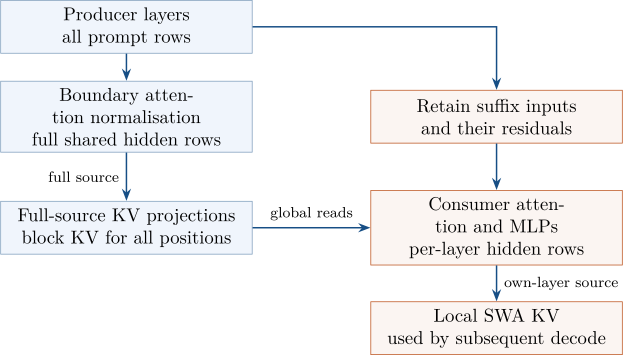
Our concrete case is a long prompt with no prefix-cache hit, processed in one chunk. We
explicitly enable compact mode. The producer layers process all prompt rows. At the boundary,
two row layouts emerge (Figure 9.1). We first follow those layouts, then examine how DeepInfer
selects the retained positions.
9.2.1 One layer performs two jobs
The Hugging Face adapter’s _n_prefill_layer returns the index of the first layer whose
compression ratio is 1. Its docstring describes that layer as part of the prefill side. The runtime
predicate includes the same index among consumers [70, 71]:
def is_yoco_consumer_layer(cfg: AttrDict, layer_idx: int) -> bool:
"""YOCO consumer layer: [n_prefill_layer, n_layer) in the main model."""
return yoco_enabled(cfg) and cfg.n_prefill_layer <= layer_idx < cfg.num_hidden_layers
The executed operations resolve the apparent disagreement. In DeepseekModel.forward, the
boundary selects a consumer metadata view and retains the original metadata for full-source
work:
consumer_metadata = input_metadata.get_consumer_view()
cross_layer_runtime.consumer_full_metadata = input_metadata
input_metadata = consumer_metadata
At this point the hidden tensor still contains the original rows. The boundary layer makes compact copies of the hidden inputs and residuals, but normalises the full inputs as well:
compact_inputs, full_inputs = compact_yoco_boundary(
hidden_states, residual, input_metadata, cross_layer_runtime, hc_enabled=self.hc_enabled
)
cross_layer_runtime.consumer_full_hidden = self.attn_norm_forward(*full_inputs)[1]
hidden_states, residual = compact_inputs
del compact_inputs, full_inputs
hidden_states, hidden_states_bf16, residual = self.attn_norm_forward(hidden_states, residual, hc_post_intervention)
consumer_full_hidden holds the full attention-normalised input. The normalisation on the
last line supplies the compact input for this layer’s attention. A few lines later, the boundary
saves the compact normalised copy as shared_hidden; the comment explicitly distinguishes it
from the full copy (lines 147–152, author’s translation) [21].
The boundary therefore supplies full shared rows and runs consumer attention on compact rows. It is not a full producer attention layer followed by a separate first consumer layer. Counting it twice would misstate both the architecture and the saved computation. Its MLP also runs on the compact rows passed through attention.
9.2.2 Block KV keeps its full source
Consumer layers that own block KV call _store_yoco_full_kv. This method reads
consumer_full_hidden into a local variable named full_hidden. It checks the row count against
full_metadata, then projects and stores the KV:
assert self.shared_hidden_kv_proj is not None
projected_kv = self.shared_hidden_kv_proj(full_hidden)
with userbuffer.cp_session(enabled=use_cp):
wait_projected_kv = _make_cp_gather_getter(projected_kv, use_cp)
pre_rope_kv = self._store_main_kv(wait_projected_kv, kv_cache, full_metadata)
cross_layer_runtime.pre_rope_kv = pre_rope_kv
Both operations cover source positions excluded from consumer attention and MLP computation. Layers that reuse another layer’s block KV need not repeat that projection. In our no-hit case, truncation has not removed the inputs required to construct block KV. This is exactness of the dependency, not a claim that every kernel layout yields bitwise-identical arithmetic [22].
There is a second kind of cross-layer sharing in the repository. SharedLayerTopology maps
layers to sources for KV, index keys, selected indices and candidate blocks. These segmented
maps are distinct from sharing the boundary representation. Its validation requires a
KV source at the YOCO boundary: a share-KV segment cannot cross that boundary
(cross_layer.py, lines 114–116). These maps govern reuse of computed entries between layers;
the shared hidden path determines the input from which those entries are projected
[72].
9.2.3 SWA keeps a per-layer dependency
In the HF adapter, yoco_swa_share_hidden is false. The local KV therefore comes from the
current hidden input. The method _project_q_and_swa selects that source alongside the query
projection:
q_a_kv_swa = self.q_a_kv_swa_proj(hidden_states)
if self.yoco_swa_share_hidden:
assert shared_hidden_bf16 is not None, f"layer {self.layer_idx}: yoco_swa_share_hidden requires shared_hidden_bf16"
return q_a_kv_swa, self.kv_swa_proj(shared_hidden_bf16)
if self.use_swa:
return q_a_kv_swa.split([self.q_lora_rank, self.qk_head_dim], dim=-1)
return q_a_kv_swa, None
With the flag false, split separates query and local KV components produced from
hidden_states. With it true, a separate projection takes shared_hidden_bf16. These
correspond to the two dependency choices in the opening experiment. In the inspected V4.1
configuration, a consumer row near the retained region’s left edge loses SWA neighbours. Its
changed output can become a later consumer’s KV input. Preserving full block KV does not
repair that local dependency.
The toy’s shared-input case explains why moving KV to a shared source can remove this particular dependency. It does not establish that enabling the flag would make DeepInfer’s whole computation exact: the rest of the model, indexing and numerical kernels would need their own checks. The engine we are reading uses the per-layer choice.
9.3 Which rows can a consumer see?
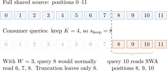
Let the prompt length be , the retained count , and the window . The retained region starts at , clipped by the actual prompt extent. For our small diagram, , , . Full-source block KV still covers all 12 positions; consumer queries retain positions 8 through 11 (Figure 9.2).
9.3.1 Compaction changes indices, not positions
The C++ function fill_yoco_truncation_metadata prepares per-request clipping and compact
query indices; update_yoco_prompt_v4 checks the keep count before calling it (lines 203 and
349–359). In a chunk starting at q_start with q_len rows, data_len is the full sequence length
used to locate the suffix:
int32_t clip_prefix = compact ? std::clamp(data_len - keep_tokens - q_start, 0, q_len - 1) : 0;
clip_prefixes[i_seq] = clip_prefix;
full_bases[i_seq] = full_base;
int32_t keep_len = q_len - clip_prefix;
p_cu_c[i_seq + 1] = p_cu_c[i_seq] + keep_len;
full_base += q_len;
For a single 12-row chunk, this removes eight rows and leaves four. For a four-row chunk covering positions 0–3 of that same prompt, it removes only three: the upper clamp is . The remaining position 3 is a placeholder, outside the final retained region. It keeps the chunk’s consumer computation nonempty; it is not another useful suffix token.
The metadata view preserves original positions while replacing query-aligned arrays and counts:
assert self.yoco_compaction_enabled
view = copy.copy(self)
qi = self.yoco_consumer_query_indices
view.total_q = self.yoco_consumer_total_q
view.cu_seqlens_q = self.yoco_consumer_cu_seqlens_q
view.positions = self.yoco_consumer_positions
view.slot_mapping_store_swa = self.yoco_consumer_slot_mapping_store_swa
view.ks = self.yoco_consumer_ks
view.ke = self.yoco_consumer_ke
view.kv_ca_index_offset_len = self.yoco_consumer_kv_ca_index_offset_len
In the one-chunk example, compact row 0 represents original position 8. RoPE positions and ring slots must follow the latter. The view also replaces SWA pivots and clears derived attention fields so they can be regenerated for the new layout. It is a shallow copy: fields that were not replaced can still share tensors with the original metadata, and the docstring forbids modifying those shared tensors in place (author’s translation) [73]. With context parallelism, further code redistributes the retained rows across ranks; the source and consumer layouts still remain distinct.
9.3.2 Three lower bounds
Keeping a row does not grant it access to every old cache entry. The decisive line in
yoco_swa_visibility is:
int32_t abs_lo = std::clamp(std::max({pos - window_size + 1, rect_lo, valid_start}), 0, pos + 1);
rect_lo is the retained-region start; valid_start is the earliest valid state position. For a query at
position ,
the lower bound is
Visible positions run from through . If , that interval is empty. The comment says that the valid-state bound prevents attention from reading zeroed slots (author’s translation, lines 151–154) [38].
For query 8 in the diagram, the usual window is 6–8 but the kept-region bound raises the start to 8. Query 10 sees 8–10, a full three-position window. Its current layer has all three positions, yet their representations may already carry earlier truncation error. This is the distinction the lab exposed. The Q&A’s expresses the replay case with a 128-position window; the code also carries the valid-state bound and the empty-interval case.
A placeholder must not overwrite live ring state. The slot assignment checks whether the position actually belongs to the retained region:
bool in_rect = pos >= data_len - keep_tokens;
if (in_rect && q_len - j <= swa_block_size)
p_slot_c[i_qc] = p_seq->state_id * swa_block_size + pos % swa_block_size;
else
p_slot_c[i_qc] = -1;
The extra length condition limits writes to the trailing ring capacity, as in chapter 5. The placeholder at position 3 receives ; an ordinary retained row uses its original position modulo the ring size. Physical bytes left from older work do not override these validity rules.
9.3.3 Modes, defaults and limits
off keeps the ordinary prefill. mask retains all query rows but narrows consumer SWA visibility.
compact uses that narrowed visibility and removes query rows, apart from placeholders. Mask
therefore supplies a comparison for the compact layout. It removes no consumer rows; only its
count of visible SWA pairs falls. The benchmark’s help text says that mask computes
every consumer token and saves no work [15]. Both enabled modes truncate the local
dependency.
The numbers governing this path have different jobs:
| Number | Meaning and evidence |
| 128 | SWA window for the V4.1 setting in the Q&A; supplied by model configuration |
| 134 | Inference ring: window plus maximum backtracking, under the chapter 3 defaults |
| 140 | README’s suggested explicit keep count for V4.1 |
| Runner assertion under those window/backtracking settings |
|
| Production prefix-hit cap in the Q&A; not a released hit-policy implementation |
|
| 2,541 / 2,560 | Derived SWA dependency span / Q&A’s conservative product |
The Q&A describes replaying 128 tokens; the README tells users to retain 140. These are
not interchangeable defaults. environ.py defaults truncation to off and the keep count to zero.
To enable it, users must supply a valid count. ModelRunner.load_model asserts that the count
covers the window plus maximum backtracking. That assertion protects capacity after
backtracking; it does not prove exact reconstruction [1, 30, 45].
Both enabled modes disable prompt log probabilities. The engine enforces this in
LLMEngine.add_request by clearing prompt_logprobs: compact omits prompt rows, and mask
changes their local context. Compact imposes two further restrictions when the YOCO path is
enabled:
if dflash_target_layer_ids:
in_consumer = [t >= cfg.n_prefill_layer for t in dflash_target_layer_ids]
assert all(in_consumer) or not any(in_consumer), (
"yoco consumer compaction requires DFlash target layers on the same side of "
f"n_prefill_layer ({cfg.n_prefill_layer}), got {dflash_target_layer_ids}"
)
self.dflash_targets_in_consumer = all(in_consumer)
assert all(layer_id < cfg.n_prefill_layer for layer_id in engram_layer_ids), (
"yoco consumer compaction does not support Engram in consumer layers yet."
)
All DFlash target layers must fall on the same side of the boundary, so its collected features have a consistent row layout. Engram layers must remain before the consumer boundary. These two checks belong to compact mode; they are not blanket restrictions on mask [20, 5].
9.4 Which state may enter the prefix cache?
Chapter 4 divided a StateBlock into stored and dropped regions. We can now explain the
consumer SWA part of that division. In worker/cache_engine.py, _is_dropped_swa_layer
returns true for layers at or beyond n_prefill_layer, provided the model has a consumer region.
It does not inspect the truncation mode. The counts use that predicate:
self.swa_num_layer = sum(int(GPUCacheInterface._has_SWA(attn_module)) for attn_module in runtime_attn_modules)
self.swa_store_num_layer = sum(
int(GPUCacheInterface._has_SWA(attn_module))
for layer_id, _, attn_module in iter_runtime_attn_modules(attn_module_list, cfg.num_hidden_layers)
if not _is_dropped_swa_layer(cfg, layer_id)
)
self.swa_drop_num_layer = self.swa_num_layer - self.swa_store_num_layer
self.swa_block_size_kvstore = get_kvstore_swa_block_size(window_size)
self.swa_block_size_inference = get_inference_swa_block_size(window_size)
Later, state_size_to_disk is assigned only the stored SWA region’s inference-layout byte
count. Consumer SWA remains in the dropped region alongside compression state. The transfer
from the prefill engine to the decode engine (PE to CE in the docstring and Q&A) includes that
region, because decode needs it. “Dropped” thus means excluded from prefix persistence, not
released at the end of prefill [23].
This policy makes the next prefill rebuild consumer SWA instead of retrieving it. With
truncation enabled, that reconstruction is approximate. With it off, consumer computation is full
only when nothing is restored. load_state_from_store_to_prefill_cache copies stored state
into a prefill slot after a hit. Its first statement asserts that truncation is not off whenever the
model has dropped SWA layers (lines 836–837). A hit without truncation would need consumer
SWA for positions before the hit, and nothing stored supplies it. The release therefore ties
restored prefix state to truncated consumer replay, although the cache partition itself is the same
in either mode [23].
The Q&A identifies the first 20 layers as the stored V4.1 layers, and the model report gives 20 encoder and 20 decoder layers. These counts are documented model settings, not numbers implied by the generic predicate [2, 69].
9.4.1 The other bounded replay
The deployment Q&A uses bounded replay for two operations. Our source path so far is the decoder operation:
| Decoder replay | Encoder replay |
|
| Trigger | Prefill with truncation enabled | Block-KV cache hit without usable SWA |
| Work | Rebuild consumer SWA over a bounded suffix | Replay the hit prefix’s last block, then process the uncached suffix |
| Evidence | Released prefill and consumer code | Q&A’s production design; released hooks without the driving hit policy |
For encoder recovery, the Q&A describes reusing the replayed prefix’s block KV without recomputing or overwriting it. Only its SWA is rebuilt; the uncached suffix produces both kinds of KV. The production cache manager chooses a block-aligned hit and backs off one block when qualifying SWA state is missing. That cache-management implementation is outside the release [2].
The released hooks support parts of such a path, but do not drive it. swa_valid_start is
initialised or reset to zero in KvCacheState; it has a binding, but the inspected Python code
contains no writer. The scheduler reserves and clears zero_states without filling it. It stores
truncate_len without reading it. Following those names alone would therefore not reconstruct
the production hit-recovery algorithm [6, 8].
The documented hit cap also leaves an integration question. Capping a hit at
guarantees
at least 134 uncached rows. Those rows could supply the shared hidden inputs needed by decoder
replay; that connection is an inference about the unreleased driver. An aligned hit exactly at the cap
leaves 134 rows, not the README’s 140. The released metadata code makes the gap concrete.
With ,
and
, the first query’s
lower bound is
unless
is raised. Its visibility therefore includes six consumer ring entries from before the hit
(start_slot is 122). Restoring a hit writes only the stored region, so nothing in the release fills
those entries. This is our reading of the metadata code; we have not executed it. Block alignment
and an SWA miss can lengthen the suffix, but neither supplies a universal answer for the
exact-cap case. The release does not establish how that service policy and the suggested keep
setting are combined. Chapter 11 will discuss the documented policy with this limit
intact.
9.5 Count the saving; choose the error baseline
python3 labs/20_replay_cost.py
The second lab translates DeepInfer’s query-range and SWA pair-count formulas into standard-library Python. It checks them against a reference that enumerates every visible query-key pair. The first examples use and :
window=3, keep=4; entries are consumer rows / SWA pairs
case           off       mask     compact
short         2/ 3    2/ 3    2/ 3
long         12/33   12/ 9    4/ 9
clipped       4/ 9    4/ 0    1/ 0
crossing      4/12    4/ 3    2/ 3
valid-start   2/ 3    2/ 3    2/ 3
The long case covers all 12 prompt positions. Full SWA has pairs. Truncating visibility leaves pairs in either enabled mode. Mask still executes 12 query rows; compact executes four. In the clipped case, the chunk covers positions 0–3. Compact executes its one placeholder with no visible SWA keys. The crossing case covers positions 6–9: only 8 and 9 remain useful, with one and two visible keys respectively. The valid-start case begins at 10 and excludes all earlier state; its two queries have one and two keys even with truncation off. These cases separate row counts from attention-pair counts.
9.5.1 The estimator knows about placeholders
FlopsEstimator::query_ranges starts with the full query interval
. Its
consumer adjustment follows the same chunk rule as the metadata builder:
QueryRange consumer = full;
if (is_prompt && (compact || has_truncated_swa)) {
const int cutoff = full_len - keep_tokens;
// A fully clipped compact chunk still executes its last query row.
if (compact)
consumer.begin = std::clamp(cutoff, start, k - 1);
const int swa_start = std::max(swa_valid_start, cutoff);
consumer.swa_pairs =
window_size > 0 ? pairs(std::max(0, consumer.begin - swa_start), std::max(0, k - swa_start), 1, window_size) : 0;
}
return {full, consumer};
pairs uses a prefix sum. For a window ,
the cumulative pair count through
positions is
Subtracting two prefix counts gives an interval’s work. Subtracting swa_start first expresses
the interval relative to its valid local source; clamping to zero handles queries before that source.
The lab compares these formulas with direct key enumeration on 8,910 cases, including short
sequences, chunk boundaries and nonzero valid starts.
A 1,024-position prompt processed in four 256-position chunks illustrates why keep count alone is insufficient. With , the first three chunks each execute one placeholder consumer row and the last executes 140. The total is 143, whereas one full chunk executes 140 consumer rows. The source estimator counts the extra rows even though they have no visible SWA keys.
9.5.2 Why the saving can approach one half
Ignore differences in layer cost for a moment. For producer layers, consumer layers and one prefill chunk, the ratio of retained layer-row work to full layer-row work is
V4.1 has equal halves: the model report gives 20 encoder and 20 decoder layers [69]. With and much larger than , the ratio approaches one half. The lab’s illustrative equal-cost calculation gives:
Equal layer costs, 20 producer + 20 consumer layers, keep=140
length    full row-work    compact row-work    ratio
    64             2560                2560   1.0000
  1024            40960               23280   0.5684
 16384           655360              330480   0.5043
At length 64 there is nothing to remove. At 1,024, the ratio is about 0.5684; at 16,384 it is about 0.5043. This explains the scale of the Q&A’s “nearly halving” claim, rather than reproducing a model-specific FLOP count.
DeepInfer’s actual estimator retains work that the row proxy omits. calc_kproj_flops takes
the full query range for block-KV projections. calc_attn_flops combines full and consumer row
terms, SWA pair terms, and global-attention pair terms. The boundary normalisation-related
contractions also retain full-row work. calc_non_attn_flops weights producer and consumer
rows using their own coefficients. Chapter 2’s FP8-equivalent accounting still applies; these counts
do not turn directly into execution time [14].
The repository’s tests/engine/test_flops_estimator.py compares the native estimator
with per-layer, per-query accounting, including off, mask, compact and chunk cases. It requires
model metadata and the compiled extension. Our lab checks the translated range and pair
formulas, not that native test or the full model’s cost [74].
9.5.3 Equivalence needs the right comparison
The opening experiment compares shortened computation with full computation. The released YOCO checks ask a different question: does compact match mask? Their L1 check compares metadata, visible keys and slots. L2 compares model log probabilities and top-token results along a fixed teacher-forced trajectory. Both modes use truncated SWA, so agreement between them cannot establish that truncation preserves the full model [75].
The script also supports an untruncated baseline by setting keep_tokens=0; it then
selects off. The capability to produce a baseline is not a published error measurement.
No full-versus-truncated error measurement was found in the inspected release. The
model report states that the reconstructed decoder SWA KV is not mathematically
equivalent to a full decoder pass. It reports a negligible effect on response quality, and
simulates the same replay during post-training [69]. These are the authors’ findings, not
an error bound reproduced here. The last point means the approximation is partly a
model property: post-training adapted the model to it, so it is not only an engine
shortcut.
An evaluation of the approximation would hold inputs and the continuation trajectory fixed, then compare full and truncated intermediate state and log probabilities. A separate task evaluation would ask whether those differences matter to answers. Exact state equality, numerical agreement, and acceptable model quality are three different claims. Chapter 10 returns to the contracts checked by the released equivalence tests.
9.6 Experiments to try next
- Use equation (9.1) for four layers and a five-position window. List the intervals required at each layer to recover the final window. Which number counts input positions, and which counts layer-row computations?
- In lab 19, retain four inputs instead of three or five. Find the first differing second-layer cache entry. Is the final prefill result exact? Check one subsequent decode step as well.
- A prompt has 12 positions, keep count four and window three. For a chunk covering positions 4–7, find the compact query, its SWA visibility and its write slot. Explain why a query can execute without updating the ring.
- Switch truncation from compact to off. Does
_is_dropped_swa_layermove consumer SWA into the stored region? Trace where that state is still needed before it can be released. Then follow a prefix hit intoload_state_from_store_to_prefill_cache. Why must it refuse to run? - A block-aligned hit leaves 134 uncached rows. Which part of a 140-row retained suffix lies before the hit? Identify the released evidence and the missing service behaviour needed to say how those rows are supplied.
- Mask and compact produce identical log probabilities. State what this establishes and propose a different comparison for the approximation error.