CHAPTER 08

Spend verification work wisely

Chapter 4 reserved room for draft tokens: cheap guesses that the model checks in its next decode step. Chapter 3 counted the six query positions that such a step evaluates, and chapter 6 corrected the host’s lengths once the device knew how many guesses survived. Two questions remain. What makes keeping a guess legitimate when we sample rather than always choose the most likely token? And how many guesses are worth the work of checking? The first is a question about probability, the second about cost. DeepInfer answers both in code that runs at every decode step. The README calls this feature DSpark and confidence-scheduled verification; the deployment Q&A explains how DSpark uses predicted acceptance to allocate a variable verification budget [1, 2].

python3 labs/17_verification.py

The experiment enumerates three possible tokens with exact fractions. The target distribution is the one we want; the draft distribution belongs to the cheaper predictor. The standard column uses an exact correction rule. The penalised column changes that correction, using an exaggerated penalty so that the difference is visible:

Exact probabilities; illustrative alpha=9/10
token  target  draft  standard  penalised  difference
  A     1/2    1/3       1/2      19/39      -1/78
  B     1/3    1/2       1/3        1/3          0
  C     1/6    1/6       1/6       7/39       1/78
Standard output equals target; penalised output obeys both bounds.

The standard rule recovers the target exactly. The modified rule moves $1∕78$ of probability from A to C. Both columns sum to one, and both accept proposed tokens using the same test. The difference comes from what happens after a rejection. DeepInfer uses this second kind of correction, with a much smaller penalty. Understanding that choice comes before deciding how much verification work to schedule.

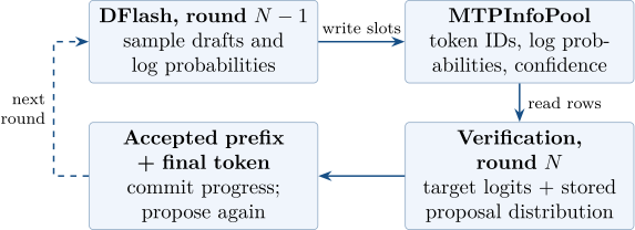
Figure 8.1 locates the two decisions in DeepInfer’s loop. DFlash, DeepInfer’s draft model, proposes tokens; a pool retains them with their proposal probabilities and confidence estimates. The next verification step reads that proposal, but may check only a prefix. We first explain acceptance and correction, then the budget, and finally which round supplies each piece of information.

8.1 Accept or correct

Write $P(x)$ for a target probability and $Q(x)$ for the probability with which the draft actually proposes token $x$. Draw from $Q$, then accept the proposal with probability

We only need this ratio for tokens that can be drawn: $Q(x)>0$. The accepted probability mass at token $x$ is therefore $\text{min}(P(x),Q(x))$. Where the draft offers too much mass, the test removes the excess. Where it offers too little, acceptance alone cannot fill the gap.

Set $s(x)={[P(x)-Q(x)]}_{+}$, where ${[z]}_{+}=\text{max}(z,0)$, and let $\mathrm{\Delta }={\sum }_{x}s(x)$. Since both distributions sum to one, $\mathrm{\Delta }$ is also the total rejection probability. On rejection, draw a replacement from $s∕\mathrm{\Delta }$. The resulting probability of token $x$ is

If $\mathrm{\Delta }=0$, every proposal is accepted and no replacement is needed. This is the probability argument behind the standard speculative sampling algorithms of Leviathan, Kalman and Matias and of Chen and colleagues [56, 57].

In our example, the accepted masses of A, B and C are $1∕3,1∕3,1∕6$. Only B can be rejected: it is proposed with probability $1∕2$ and accepted with probability $2∕3$, leaving total rejection mass $1∕6$. Only A has a positive residual. Sending every rejection to A gives $1∕2,1∕3,1∕6$, the target distribution. Notice that the replacement need not be another draw from the target itself; it must fill precisely the missing mass.

The lab enumerates every branch. Here residual has already been formed and mass is its sum:

22    for token, q in enumerate(draft):
23        if not q:
24            continue
25        accept = min(F(1), target[token] / q)
26        output[token] += q * accept
27        rejected = q * (1 - accept)
28        if rejected:
29            assert mass > 0
30            for replacement, weight in enumerate(residual):
31                output[replacement] += rejected * weight / mass
32    assert sum(output) == 1
33    return output

The full lab checks equality on a grid of three-token distributions with probabilities in sixths. The grid includes identical distributions, disjoint supports and zero probabilities. These are exact calculations, not a histogram from a finite sample. The derivation explains why equality holds generally under the stated assumptions; the grid checks the implementation on those cases.

For a draft prefix, apply the argument at each position conditional on the prefix already accepted. A target forward pass can compute the distributions for several positions together. If a draft is rejected, emit its replacement and discard later candidates: their target distributions were evaluated after a prefix we did not keep. If all checked drafts are accepted, emit one further target sample. Thus checking $k$ drafts can yield up to $k+1$ tokens. Stopping conditions can shorten the published result. Exact one-position correction does not, by itself, prove every adaptive choice of which positions to check.

8.2 What DeepInfer verifies

Chapter 6 followed the worker from forward to sampling. Inside that sampling stage, Sampler._verification maps flat logit rows to requests and local positions. It marks the first $q-1$ rows of each request for draft verification; the final row is the extra target sample if the prefix survives. The CUDA metadata helper expresses this as step + 1 < length [58].

The verifier needs the distribution that produced the previous draft, not a new prediction of that distribution. Its call to process_sampling receives stable pool storage and a row mapping:

439(
440    logprobs,
441    token_index_cur,
442    candidate_token_ids,
443    accept_result_verify,
444    draft_selected_logprobs,
445    accept_probs,
446) = process_sampling(
447    logits,
448    driver_inputs.kernel,
449    self.force_topk,
450    row_to_req=row_to_req,
451    local_step=local_step,
452    is_verify=is_verify,
453    last_nextn_token_logprobs=mtp_info_pool.logprobs if speculative_inputs is not None else None,
454    last_nextn_token_logprobs_index=mtp_info_pool.logprobs_index if speculative_inputs is not None else None,
455    draft_token_ids_pool=mtp_info_pool.token_ids if mtp_info_pool is not None else None,
456    mtp_info_read_rows=speculative_inputs.mtp_info_read_rows if speculative_inputs is not None else None,
457)

The read-row mapping selects the stored proposal for each verification row. The helper process_sampling, in layers/sampler_utils.py, transforms the target logits and invokes the sampling kernel. In force_topk mode it first selects a smaller vocabulary and remaps the stored draft probabilities into the target’s selected vocabulary. The optional index pool preserves the connection to original token IDs. A missing draft token cannot be treated as if it had an arbitrary index in that smaller space [59].

Here and below, $P$ means the target distribution after the applicable sampling transforms, including temperature and top-k/top-p filtering. It is not necessarily the raw model softmax. Likewise $Q$ must be the distribution used to sample that draft. Structured-output masks are applied before this call, and golden overrides can later replace results. We analyse stochastic verification without such overrides; chapter 10 treats their separate contracts.

8.2.1 The acceptance test is standard

The CUDA kernel reads the target and stored draft log probabilities. After accounting for target filtering, it performs this test:

391accept_lp = T.min(target_lp - draft_lp, T.cast(0, T.float))
392verify_seq = sample_positions[row] * 3 + 2
393T.rng_init(seed_val, verify_seq)
394accepted_s[0] = T.rng_rand_float(32, "uniform") < T.exp(accept_lp)

Exponentiating the minimum gives $\text{min}(1,P∕Q)$. The random stream uses the request’s seed and a value derived from the sampling position, rather than the decode step number. That choice matters when batching changes, but it is only one part of a deterministic execution contract.

8.2.2 The correction deliberately leaves a small bias

Further down the same kernel, replacement weights are formed differently from the standard residual:

438    for j in T.Parallel(SAMPLE_BD):
439        pf[j] = T.Select(
440            i0 * SAMPLE_BD + j < vocab_size,
441            T.max(pf[j] - T.exp(draft_lf[j] - DRAFT_PROB_PENALTY), 0.0),
442            0.0,
443        )
444if do_sample:
445    accumulate(sample_cfg, pf, sample_acc_frag)

DRAFT_PROB_PENALTY is $5\times 10^{-5}$. Its comment says that the penalty prevents rejection sampling from finding nothing to sample (author’s translation of tilelang_ops/common.py, line 53). Writing $\alpha =\text{exp}(-5\times 10^{-5})$, these weights are

Reducing the subtracted draft probability adds residual mass. It can give a token a positive replacement weight even when its standard residual is zero. In the lab, $\alpha =9∕10$: A’s residual becomes $1∕5$, C’s becomes $1∕60$, and B’s remains zero. Rejection still occurs with probability $1∕6$. Normalising those new weights gives A $12∕13$ and C $1∕13$ of the replacements, explaining the transfer of $1∕78$.

The source docstring gives a bound for this modified rule. It names the draft $p$ and the target $q$; our notation reverses those roles, using $Q$ and $P$. Its argument, rendered here in the book’s notation (author’s translation), starts by writing

The added mass satisfies $0\le d(x)\le \mathit{𝜀Q}(x)$, so $D\le 𝜀$. With the unchanged acceptance test,

For the upper bound, $d(x)\le \mathit{𝜀P}(x)$ also holds: check separately $P(x)\ge Q(x)$ and $P(x)<Q(x)$. Hence $A(x)-P(x)\le d(x)\le \mathit{𝜀P}(x)$. For the lower bound, use $s(x)\le \mathrm{\Delta }$, $D\le 𝜀$ and $\mathrm{\Delta }\le 1$ to obtain $P(x)-A(x)\le D\mathrm{\Delta }∕(\mathrm{\Delta }+D)\le 𝜀∕(1+𝜀)$. The no-rejection case is immediate. Together these give the docstring’s per-token bound [60]:

Lab 17 checks both inequalities for four rational values of $\alpha$ on the same distribution grid:

Exact grid: 3136 bound checks (includes equal and disjoint supports).
Configured penalty=5e-5: epsilon approximately 0.0000499988

The rational $9∕10$ makes the difference visible and exactly computable. The configured exponential is not a rational number; its displayed $𝜀$ is a decimal approximation. These calculations verify the idealised rule. The general bound comes from the argument above, not from the number of examples tried.

There is a further implementation boundary. accumulate converts the weights to fixed-point integers before summing them. If the accumulated replacement mass is zero, lines 506–518 of the kernel fall back to the first token attaining the maximum logit. Floating-point probability transforms, fixed-point accumulation and that fallback are not covered by the docstring’s ideal-arithmetic bound. For example, in exact arithmetic with $\alpha <1$, ${\sum }_{x}r(x)\ge 1-\alpha >0$; the zero-mass fallback is not a branch that our rational model should invent. We have inspected these implementation choices, not established a combined error bound for the GPU kernel [58, 61].

This is the chapter’s comparison boundary: DeepInfer retains the standard acceptance rule and modifies the rejection residual. The inspected code and its comment support that difference. They do not support a claim that the released sampler preserves the target distribution exactly.

8.2.3 Only a surviving prefix is published

Some sampled candidates follow a rejected draft and cannot be published. The helper get_accept_result finds which remain usable. After identifying the request and its first row, the kernel scans earlier positions:

261req = T.alloc_var(T.int32, row_to_req[row])
262start = T.alloc_var(T.int32, ftp[req])
263alive = T.alloc_var(T.bool, True)
264prev = T.alloc_var(T.int32, start)
265while alive and prev < row:
266    prev_accept = T.alloc_var(T.bool, raw_accept[prev])
267    if has_golden:
268        prev_golden = T.alloc_var(T.int32, golden[prev])
269        if prev_golden != -1:
270            prev_draft_row = T.alloc_var(T.int32, read_rows[prev])
271            prev_accept = prev_golden == draft_token_ids_pool[prev_draft_row]
272    alive = is_verify[prev] and prev_accept
273    prev += 1
274token_ids_out[row] = token
275accept_out[row] = alive and is_verify[row] and accept
276is_final_out[row] = alive and (not is_verify[row] or not accept)

Ignoring the explicit golden overrides, alive remains true only through an accepted draft prefix. The first rejection is a final row; later rows are neither accepted nor final. If no draft rejects, the extra, non-verification row is final. finalize_verification collects that final token and the accepted draft IDs. Suppose four positions checked three drafts and the second draft failed. The first draft and the second row’s replacement survive; the third draft and extra target sample do not. Chapter 4’s processed-token count is later corrected to this actual progress, even though the forward already evaluated and wrote state for more positions.

8.3 How many positions are worth the work?

python3 labs/18_verification_budget.py

Lab 18 translates DeepInfer’s CPU budget search and checks it against exhaustive prefix choices on a small input. There are two requests, each with three available drafts. Their older cumulative confidence values are $(0.90,0.72,0.36)$ and $(0.80,0.40,0.10)$. The first request’s raw estimates were $(0.90,0.80,0.50)$: reaching draft 3 requires accepting drafts 1 and 2, so the estimated chance of keeping the prefix is their product, $0.36$. These are predictions, not the acceptance probabilities computed by verification.

The lab forms the prefix products with itertools.accumulate, using multiplication:

20def cumulative(raw):
21    assert all(0 <= r <= 1 for row in raw for r in row)
22    return [list(accumulate(row, mul)) for row in raw]

The script prints every candidate under four assigned cost curves. Here is the staircase case:

stairs: synthetic time units; sampler=2, slope=0
  positions graph expected time  output/time
          2     2     2.00   10       0.2000
          3     4     2.90   12       0.2417
          4     4     3.70   12       0.3083
          5     6     4.42   14       0.3157
          6     6     4.82   14       0.3443
          7     8     5.18   30       0.1727
          8     8     5.28   30       0.1760
  chosen total=6, q(N-1)=[2, 4]
  allocation using N-2 instead: [3, 3]

There is one main input position per request before adding any drafts. Start with two expected output tokens and two positions. Sorting all cumulative values gives $0.90,0.80,0.72,0.40,0.36,0.10$. Taking the first four extras raises the score to $2+0.90+0.80+0.72+0.40=4.82$, with six positions of work. The assigned cost is 14, so the score is $4.82∕14\approx 0.3443$. A seventh position crosses a graph boundary and costs 30; its extra expected output cannot pay for that jump. Figure 8.2 shows the three assigned cost curves.

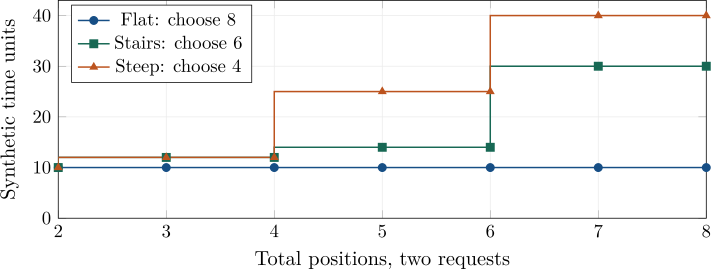
Changing only the cost curve changes the winning total: flat costs choose all eight positions, the staircase chooses six, and the steep curve chooses four. In the fourth case, moving the steep curve’s second graph size from four to five makes five positions best: the fifth now fits in the cheaper bucket. Within a bucket, another position with positive expected value improves the score at no extra modelled time. This is chapter 2’s distinction between request count and evaluated positions expressed through graph sizes.

The script also changes the confidence history used for allocation. In the staircase output, the total is six but the lengths are $[2,4]$; allocating with the older values would give $[3,3]$. The total and its distribution are separate decisions. We will trace their rounds after inspecting the search.

8.3.1 A search over totals, then a second allocation

The decode scheduler calls MTPVarlen::schedule after choosing requests. It sums the returned query lengths into num_batched_tokens. Here bsz counts positions, not requests. The class builds two sorted queues of cumulative confidence values, one to choose this total and one to divide it among requests. Its comparator sorts by descending value, breaking ties by request index (lines 210–214) [62].

For estimates in $[0,1]$, cumulative values along a request never increase. A later position cannot strictly outrank an earlier one. Equal values need not retain position order in the C++ sort: the result stores a count per request and uses that many positions from the beginning. Thus counts still specify prefixes. This is why cumulative estimates, rather than unmultiplied per-position confidence, fit this allocation rule.

For each total, the search scores the smallest graph large enough:

234int cur_bsz_idx = 0;
235auto update_best = [&]() {
236    while (cur_bsz_idx < num_bsz_selections && cur_bsz > _decode_perf_curve[cur_bsz_idx].first) {
237        ++cur_bsz_idx;
238    }
239    if (cur_bsz_idx == num_bsz_selections) {
240        return;
241    }
242    const auto &[graph_size, baseline_ms] = _decode_perf_curve[cur_bsz_idx];
243    const double time_ms = baseline_ms + slope_ms * graph_size + sampler_ms;
244    const double cur_throughput = cur_expected / time_ms;
245    if (cur_throughput > best_throughput) {
246        best_throughput = cur_throughput;
247        best_bsz = cur_bsz;
248    }
249};

There are three terms in time_ms: a startup forward measurement for the graph, an online slope times the graph size, and an estimated sampler time. Before this excerpt the slope is clamped to zero or above. Candidates beyond the largest available graph are ignored. The strict > keeps the earlier, smaller total when two scores tie.

The loop adds one candidate’s estimated output and one position at a time:

252update_best(); // All the golden tokens
253
254for (auto &acc : acc_queue_for_bsz) {
255    cur_expected += acc.first;
256    cur_bsz += 1;
257    update_best();
258}

The final allocation deliberately uses the other queue:

263seqlens_q.assign(num_seqs, 1);
264for (int i = 0; i < best_bsz - num_seqs; ++i) {
265    seqlens_q[acc_queue_for_seqs_q[i].second] += 1;
266}

Lab 18 preserves these decisions, including the tie rule, graph limit and non-negative slope. Its independent check enumerates every possible pair of prefix lengths under the older confidence values and confirms the winning total. It also tests nonzero slopes, absent drafts and equal scores. Fractions remove rounding ambiguity in the teaching input; the production search uses floating-point values. The check does not say that the newer allocation maximises the older score, or that either predicts measured throughput exactly. EOS, confidence errors and changes in workload can all separate the estimate from useful published output.

8.3.2 The engine supplies the time model

ModelRunner.profile_decode_perf measures the startup curve, if a cached curve is unavailable. It replays each captured graph once to warm up and five times with CUDA timing events. Expert routing is forced random during profiling. With NUM_TRIM=1, the sorted measurements lose one value at each end:

617times_ms.sort()
618trimmed = times_ms[NUM_TRIM : NUM_MEASURE - NUM_TRIM]
619avg_time_ms = sum(trimmed) / len(trimmed)
620sum_time = torch.full((1,), avg_time_ms, dtype=torch.float32, device="cuda")
621dist.all_reduce(sum_time, op=dist.ReduceOp.SUM, group=group)
622avg_time_ms = sum_time.item() / group.size()
623results.append((batch_size, avg_time_ms))

For five assigned times $9,10,11,12,40$, this rule gives 11. It does not average the best four, nor does it describe the maximum rank time. The cached startup curve is a baseline; current context lengths and routing can change forward cost [63].

Chapter 6 already located the device events and the wait before post-processing. The feedback connection is now visible in LLMEngine.post_process:

995if step_state.forward_events is not None and step_state.sample_events is not None:
996    # Worker has synchronized this step's sample_end_evt before calling post_process.
997    self.scheduler.update_mtp_runtime(
998        len(seq_metadata_list),
999        step_state.graph_size,
1000        step_state.forward_events[0].elapsed_time(step_state.forward_events[1]),
1001        step_state.sample_events[0].elapsed_time(step_state.sample_events[1]),
1002    )

update_runtime compares forward time with the baseline at graph size $g$, storing the normalised residual $(T_{\mathrm{forward}}-T_{\mathrm{startup}}(g))∕g$. ForwardRuntimeEstimator keeps 5,000 steps. It takes a median within each graph size having at least ten samples, then a median across those graph-size medians. A frequently used graph does not gain extra votes in that second median. This is a robust residual-slope estimate, not a least-squares fit. If no graph meets the threshold, the slope is zero. The schedule clamps a negative estimate to zero, making the startup curve the lower bound on estimated forward cost [62].

Sampler time has no startup curve. Its estimator keeps nine observations and requires five before returning a median. The search prefers history for the same request count, then a global sampler history, then zero. For example, a forward baseline of 10 at $g=6$, an estimated slope of $0.5$, and a sampler estimate of 2 give $10+0.5\times 6+2=15$ in consistent time units. The lab assigns these inputs; it does not reproduce startup profiling or measure a device.

8.3.3 Fixed length is the default

Variable-length verification is off by default: DEEPINFER_ENABLE_MTP_VARLEN is false. The draft limit is five, set by DEEPINFER_USE_NEXTN_DECODE. The actual fixed-length branch in MTPVarlen::schedule is an empty performance curve: each request receives one plus its available draft count (lines 152–157). WorkerBase.warm_up_model obtains a curve only under the graph and variable-length conditions in worker/base.py, lines 275–281. Turning on the flag alone does not guarantee a usable curve [30, 63].

With five available drafts, fixed verification evaluates six positions per request. Chapters 3 and 6 have already traced those positions through decode SWA writes and lagging metadata. Variable verification changes which prefix is evaluated; it still needs the same attention and lifetime rules.

8.4 Which round supplies the confidence?

Call the current verification step $N$. Its draft was produced in round $N-1$. That draft has three different kinds of associated information: its token IDs, the log probabilities of the distribution used to sample it, and a confidence head’s estimates of acceptance. The first two drive sampling correctness. The third predicts where verification work will be useful. Return to Figure 8.1: we can now follow the writes and reads behind its pool boundary, then distinguish the histories used by scheduling.

8.4.1 Produce once, store the distribution, verify later

DeepInfer’s draft model is the DFlash module in model_executor/models/mtp/, named after multi-token prediction (MTP); nextn is its configured draft count. DFlash starts from $[\mathrm{golden},\mathrm{noise},\dots ]$, where the first token is the just-selected target output. Its draft layers process these positions together, and sample_drafts computes base logits for them. It then samples position by position. An optional Markov correction changes the logits using the previous draft token (lines 308–314). This permits a parallel base computation while retaining that dependency during sampling [64].

The confidence head runs before sampling the token at that position. The sampling call also writes the log probabilities actually used:

315if confidence_rates is not None:
316    self.confidence_head(
317        hidden_states_before_norm[step_i :: self.max_MTP_value],
318        w1,
319        out=confidence_rates[:, step_i],
320        step_i=step_i,
321    )
322_, token_index_next, draft_token_ids, _, _, _ = process_sampling(
323    logits,
324    SamplingKernelInputs(
325        sampling_input.kernel_inputs.logits, sampling_input.kernel_inputs.seq_seeds, sample_positions_table[step_i]
326    ),
327    self.force_topk,
328    logprobs_out=next_n_token_logprobs[:, step_i],
329    tag="mtp",
330)

The same request sampling parameters feed this call, but the logits come from the draft model. Equal parameters do not mean equal distributions. With force_topk, sampled indices are mapped back to token IDs and the index mapping is retained. After the position loop, all proposal data is stored:

339self.mtp_info_pool.store(
340    sampling_input.mtp_info_write_slots,
341    prediction,
342    next_n_token_logprobs,
343    next_n_token_logprobs_index,
344)
345return prediction

MTPInfoPool owns GPU arrays for IDs, log probabilities, optional confidence and optional top-k indices. Each slot has nextn rows; slot zero is reserved for padding. The scheduler assigns slots, and verification’s read-row mapping selects their contents. This closes the path back to the pool inputs printed earlier. Recomputing a draft distribution later with different filtering would not justify the probability argument [65].

Host post-processing separately updates the confidence history in process_MTPInfo. It moves accept_rates into prev_accept_rates, multiplies the new raw confidence values along each prefix, and stores those products as the new accept_rates (scheduler.hpp, lines 1239–1250). Despite their names, these fields contain confidence-head estimates. They are not the verifier’s measured accept_probs values.

8.4.2 Choose a total with older information

Two counters locate the host’s history: schedule_cnt advances on scheduling; process_cnt advances when processing MTP information. The budget selector checks that the host is either caught up or one step behind. Its comment specifies this division of rounds (author’s translation of mtp_varlen.hpp, lines 159–167):

In code, post_process_paired is the equality of the two counters. Line 204 chooses prev_accept_rates when they match and accept_rates when they do not, supplying $N-2$ to the budget queue in either case. Line 207 always supplies the current host accept_rates to the allocation queue. That second queue is current enough without ZOS, but one round stale with it [62, 6].

The comment begins with a stronger constraint than a timing observation: confidence at later positions must not affect whether an earlier draft token is verified (author’s translation of line 159). Later confidence may depend on earlier sampled tokens, so using it to decide whether to keep those tokens can introduce selection bias. The code documents this concern and its choice of rounds; it does not provide a complete proof for the adaptive policy. Keeping the total-budget rule consistent with and without ZOS is a plausible additional reason for using $N-2$, but that is an inference, not a stated explanation that replaces the constraint.

The inspected construction appears to respect that constraint. We state the argument as an inference, not a proof. Take draft position $i$ of one request. First, the DFlash loop runs the confidence head before sampling the token at that position, so $c_i$ can depend on earlier draft tokens through the Markov input but not on $x_i$ itself. Second, cumulative values never increase along a request, and the allocation records counts, so the request’s later positions cannot take a slot ahead of $i$. Third, competing positions from other requests depend on their own drafts, not on this request’s $x_i$. Finally, the total comes from round $N-2$, before these drafts existed. Whether $x_i$ is verified may therefore depend on the prefix before it, but not on $x_i$ or later tokens of the same request.

Given an accepted prefix, $x_i$ is then a draw from $Q$ that the test either accepts or replaces. If verification stops before $x_i$, the final row is a target sample instead. In ideal arithmetic with the standard residual, both routes give the target’s conditional distribution at that position. A complete argument for the engine would also need to cover structured-output masks, golden overrides, the penalised residual and numerical effects.

8.4.3 Reallocate on the device without changing the total

In ZOS, Worker._correct_seqlens_qk receives the CPU’s fixed total_q. If the current batch overlaps the previous one, it passes the remap and the previous sampler’s device confidence to the GPU length helper. Those device values belong to $N-1$, even though host post-processing has not yet published them. The kernel first makes cumulative rates:

26# Phase 1: compute cumprod, reading confidence rates via remap (0.0 for fresh seqs)
27with T.Kernel(num_seqs, threads=128) as pid:
28    acc = T.alloc_var(T.float32)
29    acc = 1.0
30    T.pdl_sync()
31    prev_idx = remap[pid]
32    if prev_idx == -1:
33        acc = 0.0
34    for j in T.serial(nextn):
35        if prev_idx != -1:
36            acc = acc * prev_confidence_rates[prev_idx, j]
37        cum_rates[pid, j] = acc

Each position then counts how many other positions outrank it. Equal values are ordered by flat index, combining request index and position:

58# Higher rate wins; tie-break by flat index (lower index wins)
59for j in T.serial(nextn):
60    my_flat_idx = T.alloc_var(T.int32)
61    my_flat_idx = pid * nextn + j
62    beats = T.alloc_var(T.int32)
63    beats = 0
64    if other_rate > my_rates[j]:
65        beats = 1
66    if other_rate == my_rates[j] and other_idx < my_flat_idx:
67        beats = 1
68    rank_reducer[j] += beats

A position wins if this rank is smaller than total_q - num_seqs. The request’s query length becomes one plus its winning positions. The kernel does not rerun the time-model search. In lab 18’s staircase case, the total remains six while the newer values change the allocation from $[3,3]$ to $[2,4]$. The six evaluated positions still fit the same graph bucket.

The worker next corrects key lengths using the chosen query lengths and the previous accepted counts. It copies query lengths into pinned host memory and records d2h_evt. Forward uses the corrected device inputs. Before launching sampling, the worker waits for that copy and calls update_metadata_for_sampling_zos. This is chapter 6’s third metadata correction: the host’s initial lengths described a provisional division of work, and sampling must see the division that actually ran [66, 7].

Fresh rows need care. On the CPU, an empty rate vector is filled with ones if has_draft is true, and zeros otherwise. The predicate includes a request whose host processing is one step behind. On the GPU, an unmatched row (remap=-1) has zero cumulative confidence. But zero confidence does not force a query length of one: after all positive positions win, zero-valued positions can take the remaining slots. The scalar rank-count reference shows this with two surviving requests and one new row:

GPU rank-count reference; remap=[0,-1,1]
  total=7: q=[3, 1, 3]
  total=8: q=[3, 2, 3]
  CPU missing-rate fill=1, same total=7: q=[3, 3, 1]
  Both conserve the budget; zero confidence can receive surplus slots.

The CPU comparison deliberately supplies ones for that new row to expose the difference between the two local rules. Both allocations conserve the total. It is not a trace proving that this particular combination of host history, placeholder drafts and pool-slot validity reaches the engine. Establishing that requires following admission and proposal ownership together. In particular, _correct_seqlens_qk skips correction if there is no overlap at all. We leave the mixed-batch reachability question open rather than calling the different fill values a budget bug.

The README’s deterministic-sampling recipe requires variable-length verification to be disabled, alongside batch invariance and a fixed sequence seed. The acceptance RNG’s position-based indexing does not remove the runtime timings that influence the budget. Different measured timings could select different verification work; that is an inference about the restriction, developed with the other contracts in chapter 10 [1].

8.5 Reported gains and confidence error

8.5.1 Less verification can help or hurt

The deployment Q&A reports estimated throughput from EP64/DP64 benchmark data, comparing fixed-five verification with variable length. Lab 18 stores the six rows as sourced CSV data and recomputes the gains:

DSpark: DeepSeek's reported throughput estimates, not lab timings
  concurrency fixed dynamic gain
           16  4891    4816  -1.5%
           32  8964    9111  +1.6%
           48 12032   12467  +3.6%
           60 13730   14466  +5.4%
           72 14962   15961  +6.7%
           96 16817   18660 +11.0%

These are DeepSeek’s reported estimates, not timings from our experiment. At concurrency 16, average verified draft length falls from 5 to 4.44, while accepted length falls from 3.32 to 3.24; estimated throughput falls by about $1.5\%$. At 96, verified length falls to 3.24 and accepted length from 3.30 to 3.15, yet estimated throughput rises by about $11\%$. At the reported operating point of roughly 60 requests per rank, the table gives $14466∕13730-1\approx 5.4\%$ [2].

The lower accepted length at 96 is compatible with greater useful throughput if the step cost falls enough. Conversely, dropping positions inside a cheap graph bucket may save little time while reducing output. Our synthetic curves explain those possibilities; they neither reproduce the production workload nor isolate the cause of its gains. The decision depends on both sides of chapter 2’s ratio: useful output and elapsed time. A higher acceptance rate by itself settles neither.

8.5.2 What the confidence metric compares

The engine records avg_confidence_error. Verification adds $|\mathtt{\text{confidence}}-\mathtt{\text{accept\_probs}}|$ for every row marked for verification, and the logger divides the accumulated error by the verification count. Rows after an earlier rejection can still contribute because the mask marks evaluated verification positions, not only the emitted prefix. This compares confidence with a probability-like value, rather than a realised zero-or-one result [67].

There is a subtlety in that value. Even when a token was accepted, the CUDA kernel computes the full residual mass for the metric:

471if accepted_s[0]:
472    # accept_probs still requires the full fixed-point residual mass.
473    residual_mass = T.alloc_reducer((1,), sample_cfg.scale_dtype, replication="all")
474    T.fill(residual_mass, 0)
475    for j in T.Parallel(SAMPLE_BD):
476        residual_mass[0] += sample_acc_frag[j]
477    T.finalize_reducer(residual_mass)
478    if T.get_thread_binding() == 0:
479        accept_probs[row] = T.max(1.0 - T.cast(residual_mass[0], T.float) / sample_cfg.scale, 0.0)

This is the penalised, fixed-point residual, not the standard residual. Ignoring numerical rounding, the standard test’s acceptance probability, averaged over proposals at a fixed prefix, is $\beta ={\sum }_x\text{min}(P(x),Q(x))=1-\mathrm{\Delta }$. The logged proxy instead uses $1-{\sum }_{x}r(x)=1-\mathrm{\Delta }-D$, with a clamp at zero. Thus it can be smaller by up to $𝜀$ in ideal arithmetic. For the exaggerated lab penalty, the difference is visible:

Ideal arithmetic, before fixed-point rounding:
  mean acceptance of standard test: 5/6
  1 - penalised residual mass:      47/60
  difference:                      1/20

Neither quantity is the acceptance chance $a(x)$ of a particular token already drawn, and neither is that token’s realised acceptance outcome. Fixed-point rounding adds another distinction in the implementation. Calling the metric an exact conditional acceptance probability would lose these boundaries. Calling it the confidence error reported by this engine preserves the useful question: how well does the head predict the quantity the engine actually logs?

Verification spends work on possible future tokens. The next chapter reduces prefill work by reconstructing only a suffix of some model state. Its guarantee is different: the sampling residual’s probability bound does not bound errors in reconstructed hidden states. We must first ask which dependencies the shortened computation preserves.

8.6 Experiments to try next

1. In lab 17, use $\alpha =99∕100$. Predict the direction of each probability change before running. Check the bound and explain why the zero-rejection case needs no normalisation of a residual.
2. For one token in the opening example, calculate its acceptance chance after it is proposed, the mean acceptance over all proposals, and the logged ideal-arithmetic proxy. Which of these could equal zero or one in a single run?
3. In lab 18, raise the forward slope while keeping the startup curve fixed. Predict the winning total. Explain why the slope multiplies the graph size rather than the unpadded position count.
4. Replace the newer history with the older one. Which values in the saved output change? Explain why the total-budget search does not need to change.
5. Give the scalar GPU allocator more budget than there are positive-rate positions. Predict which zero-valued position wins first. Then identify the engine conditions that would need checking before treating that example as a reachable request trace.
6. Trace one DFlash proposal from its pool write through verification to final output. At each boundary identify the token IDs, stored distribution, confidence round and completion event. Separate a demonstrated numerical guarantee from an inference about adaptive selection or determinism.