CHAPTER 11

From an engine to a service

Chapter 10 examined correctness contracts within an engine. A service also passes requests and state between engines and storage. Those boundaries decide where work can run and what it must wait for.

Run the service experiment:

python3 labs/23_service.py

All four requests arrive at time zero. Each prompt has 1,024 tokens, of which 768 can be reused. Matching takes one time unit; prefill processes 128 new tokens per unit. Two decode workers each need four units per request. A handoff adds one unit, with no limit on concurrent transfers. These are assigned costs. The workers serve one request at a time, without batching or eviction. Prefix fetching adds no delay in either case; only the P/D handoff has an assigned transfer cost.

The first case sends every request to the worker holding the local prefix. The second lets either worker fetch that same prefix, at the same assigned cost:

Assigned time units; four requests, two P and two D workers
local affinity: P ends [3, 5, 7, 9]; D ends [8, 10, 12, 14]
shared cache: P ends [3, 3, 5, 5]; D ends [8, 8, 12, 12]
shared, no hits: P ends [9, 9, 17, 17]; D ends [14, 14, 22, 22]
shared, slower handoff: P ends [3, 3, 5, 5]; D ends [10, 10, 14, 14]
affinity, slower handoff: P ends [3, 5, 7, 9]; D ends [10, 12, 14, 16]

With local affinity, prefill finishes at 3, 5, 7 and 9. With a shared cache it finishes at 3, 3, 5 and 5. The last answer arrives two units earlier, not four: decode now makes the last pair wait. With equal handoff delays, sharing saves two units in both comparisons: 14 versus 12 with a one-unit handoff, and 16 versus 14 with a three-unit handoff. A shared cache with the slower handoff finishes no earlier than local affinity with the faster one. That comparison changes two variables: the extra transfer cost offsets the saving from sharing.

The no-hit case supplies a baseline for reuse: both prefill workers remain available, but processing all 1,024 positions per request moves the last completion from 12 to 22, with the handoff delay held at one unit.

Scope and order. We follow the deployment Q&A from prefix matching to routing, state movement and token output. Released DeepInfer code fixes the engine roles and the state layout at those boundaries. The Q&A describes the service that connects them. We then audit a published performance curve, using chapter 2’s accounting and chapter 8’s acceptance model. Our experiments calculate queues and rates; they do not run a serving cluster.

11.1 A request crosses several owners

The engine of chapter 1 was responsible for advancing requests. A service must first decide which engine should own each request and how its reusable state will reach that engine. Figure 11.1 separates the request’s route from the storage it can use. A released component does not imply that its production orchestration is also released.

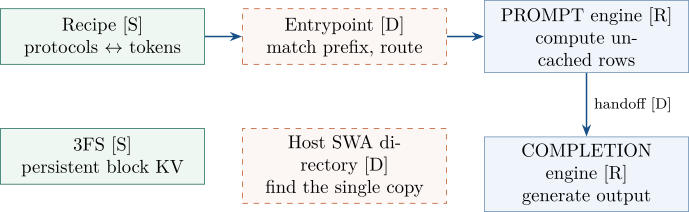
DeepInfer names the roles directly:

11NORMAL = 0  # process prompts & completions
12PROMPT = enum.auto()  # only process prompts
13COMPLETION = enum.auto()  # only process completions

A prefill engine, abbreviated PE in the Q&A, uses the PROMPT role. A decode or completion engine, CE, uses COMPLETION. NORMAL combines the two. After scheduling, the engine checks that a nonempty PROMPT step is actually a prompt step:

947if not scheduler_outputs.is_empty() and self.engine_type == EngineType.PROMPT:
948    assert scheduler_outputs.prompt_run, "Prompt engines should not perform decoding"
949    assert seq_metadata_list[0].seqlen_q > 0, "seqlen_q should be > 0"

These are executable role boundaries. They do not locate the machine-selection policy, the network transfer, or the service’s retry logic. The distinction also matters when reading benchmarks: examples/benchmark.py constructs its LLM through create_llm without overriding the engine role. It therefore uses EngineArgs.engine_type = EngineType.NORMAL, the default at deepinfer/engine/arg_utils.py:41. The examples README calls the separate prefill and decode measurements “Stage decoupling”. Those windows are inside one combined engine deployment; they are not a disaggregated P/D service [17, 15, 83].

The Q&A identifies one property shared with the DeepSeek-V3/R1 inference system: attention uses data parallelism, with equal DP and EP sizes. It also points to DualPath’s intra-group scheduling for the decode balancer, but gives no link or bibliographic reference for DualPath. These establish a stated continuity in that parallelism choice and an acknowledged scheduling precedent. The separate 3FS repository is a dependency boundary. None establishes a line-by-line derivation of the service code, which is absent here [2, 86].

Image requests add an encoder before prefill: the Q&A describes E/P/D separation. Its vision-encoder balancer first chooses a machine randomly, then chooses the GPU with the fewest assigned patches, counting width and height in patch units. Recipe handles the API-to-model representation. This adds a workload and a queue to the map, without changing why prefill and decode need different capacity signals [2].

11.2 Hits decide prefill demand

A prefix hit is useful before any bytes move. The Entrypoint matches a hash chain against metadata in the local kvcache-store’s CHECK role. A hash chain identifies a block together with its preceding prefix, so reuse concerns a matching history, not just an equal block of tokens. The resulting hit length determines how much prompt work remains. Routing needs that answer; the Q&A explicitly says matching cannot be hidden [2].

For prompt length $L$ and computation resuming at $H$, let $q=L-H$. Chapter 5’s documented quota model estimates work from the new positions $q$ and their existing context $c$. The service can then choose a prefill tier, an engine with quota left, and a rank within it:

The quota fit and its service driver are described in the Q&A, not implemented in the released scheduler. A cache hit also leaves context to read; reducing new positions does not remove all attention work.

The storage placement changes a routing constraint. With block KV in a separate shared cluster, every prefill engine can hit any prefix. It need not wait for the compute machine that produced that prefix. This is the Q&A’s reason for having no prefix-affinity routing.

Our lab holds the prefix and fetch costs fixed and changes only the eligible workers:

19    for request in range(4):
20        candidates = range(2) if shared else [0]
21        rank = min(candidates, key=lambda i: (prefill_free[i], i))
22        start = max(1, prefill_free[rank])  # matching completes before routing
23        end = start + (1024 - hit) // 128
24        prefill_free[rank] = end
25        prefilled.append((end + transfer, request, rank, start, end))

A local-cache service could instead route to an idle worker and recompute the prefix. That is another policy, not tested by the affinity case. Real shared storage pays for fetching and can itself queue. The experiment isolates the benefit of removing ownership affinity; it does not predict that shared storage always wins.

11.2.1 From work to a capacity estimate

Let $\lambda$ be requests per second, $L$ their fixed input length, $O$ their fixed output length, and $h$ the fraction of input tokens reused. Suppose $v_P$ and $v_D$ are sustained per-GPU rates for this workload. At a target utilisation $u$, a simple capacity estimate is

This linear teaching model suppresses context-dependent cost, batch shape and EP group granularity. Its units are GPU equivalents, not deployable group sizes. Lab 23 assigns $\lambda =4$, $L=1024$, $O=64$, $v_P=2048$, $v_D=128$ and $u=0.8$:

Capacity model (GPU equivalents, not deployment sizes):
reused input fraction 0%: P=3, D=3
reused input fraction 75%: P=1, D=3

The arithmetic moves prefill from three GPU equivalents to one. Output work stays at 256 tokens/s, so the decode estimate stays at three. That conclusion holds the arrival rate, output lengths and decode rate fixed. Faster prefill can still change when requests reach decode, as the opening experiment showed. It can also change achievable batching and latency. Production sizing cannot replace those effects with a constant $v_D$ without checking the workload.

The meaning of $h$ matters. One hundred requests might all hit ten tokens of a thousand-token prompt: the request hit rate is 100%, but only 1% of input tokens are reused. The Q&A sizes prefill from non-cached tokens and decode from running requests. It reports that shortening chatbot retention from seven days to about three costs 0.5–1% of KV-cache hit rate. It does not specify here whether that is a relative loss or a loss in percentage points, or give the corresponding uncached-token demand. Neither should be silently substituted into our formula [2].

Matching is on the routing path; fetching has a different dependency. The Q&A describes a separate process fetching block KV from 3FS into host shared memory, followed by an engine thread swapping it into device memory. Per-layer host-to-device copies can overlap forward computation once the needed state is ready. It describes using an RDMA network interface for these transfers through PCIe, avoiding GPU compute cores. This is a documented transfer design, not a path implemented by our queue simulator [2].

11.3 State lives in three places

Chapter 4 separated block KV from per-request state. At service scale these objects also have different homes and failure modes (Table 11.2).

The Entrypoint maintains an in-memory directory for the single host copy of SWA. A cross-machine hit pulls that state over the network. Host restart or eviction can therefore remove SWA while the block KV still exists. This is a normal trigger for chapter 9’s encoder replay, distinct from decoder replay on every truncated prefill. The Q&A also says decode KV is written to storage for later reuse, but active decode does not use KV offloading [2].

11.3.1 The released handoff layout

A completion engine needs enough state to continue immediately. A future prefix hit needs only the stored region; chapter 9 explained why consumer SWA can be dropped from that cache entry. The released helper exposes this distinction through TO_CE. In the branch without extra prefill state, selection is a contiguous slice:

790state_size = cls.total_bytes_inference if TO_CE else cls.state_size_to_disk
791if state_size == 0:
792    return None
793src = state_cache[state_id, :state_size]
794if state_tensor is None:
795    return src
796state_tensor.copy_(src)
797return state_tensor

The live size, total_bytes_inference, includes the dropped region. The stored size, state_size_to_disk, names the prefix of that layout. Despite that identifier, the Q&A says this saved SWA goes to host memory, not to 3FS. The returned slice can alias the cache when no destination is supplied. A transport driver would have to preserve its source until the transfer finishes, using the ownership reasoning from chapters 4 and 6.

When extra prefill state is enabled, the rings need rearranging. Selection allocates the appropriate destination and passes the handoff flag through to the view builder:

799if state_tensor is None:
800    state_size = cls.total_bytes_inference if TO_CE else cls.state_size_to_disk
801    state_tensor = torch.empty(state_size, dtype=state_cache.dtype, device=state_cache.device)
802
803cache_views, tensor_views = cls._carve_state_views(state_id, state_cache, state_tensor, TO_CE=TO_CE)
804for tensor_view, cache_view in zip(tensor_views, cache_views, strict=True):
805    if tensor_view.numel() == 0:
806        continue
807    select_state_slice(tensor_view, cache_view, last_hit_position)

Inside the following if TO_CE branch, consumer SWA has already been rearranged. The remaining compression state is copied separately. The comment at line 812 says: “Consumer SWA has been rearranged by ring; copy compression state directly” (author’s translation):

813dropped_compress_bytes = cls.dropped_bytes_inference - cls.swa_drop_total_bytes_inference_pad
814state_tensor[dropped_tensor_offset : dropped_tensor_offset + dropped_compress_bytes].copy_(
815    state_cache[state_id, dropped_cache_offset : dropped_cache_offset + dropped_compress_bytes]
816)

Loading a stored prefix into a prefill slot is a different operation. Its first check rejects off truncation when the model has dropped SWA layers:

836if cls.swa_drop_num_layer > 0:
837    assert envs.DEEPINFER_YOCO_PREFILL_TRUNCATION_MODE != "off"
838if not envs.DEEPINFER_PREFILL_STORE_EXTRA_STATE:
839    if cls.state_size_to_disk == 0:
840        return
841    state_cache[state_id, : cls.state_size_to_disk] = state_tensor
842    return
843
844cache_views, tensor_views = cls._carve_state_views(state_id, state_cache, state_tensor)
845for tensor_view, cache_view in zip(tensor_views, cache_views, strict=True):
846    if tensor_view.numel() == 0:
847        continue
848    load_state_to_cache(tensor_view, cache_view, last_hit_position)

The helper either copies the stored slice or reconstructs its ring views. It does not fetch bytes from another host, select a destination engine, or rebuild the dropped consumer state. In this release, calls to these two helpers outside cache_engine.py occur in tests/worker/test_state_cache_ops.py, not in a service driver [84].

That test also gives us a narrow, useful comparator. At lines 196–211 it selects state, changes the bytes, loads them back and selects again. The final comparison is:

213reselected_swa = _stored_swa(reselected_state)
214modified_swa = _stored_swa(modified_state)
215assert torch.equal(reselected_swa, modified_swa)

_stored_swa excludes per-layer alignment padding before torch.equal. This checks a layout round trip for the tested configuration, not a network transfer or a full-model continuation. We inspected this CUDA test; the book’s standard-library labs do not execute it.

11.3.2 Retention is not one number

A retention target, a capacity calculation and an eviction rule answer different questions. The Q&A gives all three, listed in Table 11.3. There TTL means time-to-live and LRU means least recently used.

The Q&A places expiry and reclamation in 3FS’s GC, with no expiry logic in kvcache-store itself. It does not give the complete precedence rules between age and occupancy pressure. A server sized for a day’s data does not by itself promise that every object will survive for that day, or that the whole cluster retains only a day [2].

Durability and read latency are separate again. The Q&A specifies 10+2 erasure coding, tolerating two simultaneous node failures, and says a read contacts 11 storage nodes and returns after any ten replies. Coding redundancy and read fan-out are different counts. The description does not explain why that read uses eleven nodes for twelve coded fragments; we do not infer a placement rule from those numbers. Nor does storage redundancy replicate the single host copy of SWA [2].

11.4 A hit has two lengths

Suppose a prompt has $L$ tokens and block KV is available for a prefix of $C$ tokens. The Q&A caps a candidate hit at $L-134$, then queries an aligned block-KV hit $L_1$. Lab 24 makes the zero case explicit:

Here $L_1$ is the reusable block-KV length; $H$ is the length skipped by computation. The lab assumes a contiguous available prefix. An actual lookup must discover that prefix and whether the matching SWA state is present.

python3 labs/24_cache_hits.py

Assigned full block-prefix availability; columns count tokens
L     block hit L1   compute hit: SWA present / missing
128   0                 0 / 0
261   0                 0 / 0
262   128             128 / 0
390   256             256 / 128
902   768             768 / 640
1024  768             768 / 640
Checks: 69666 cases; bounds, alignment, backoff, monotonicity

For $L=902$, the cap is exactly 768. With SWA present, prefill starts at 768 and processes 134 new positions. Without it, prefill starts at 640. The interval $[640,768)$ reconstructs encoder SWA; its block KV is already available and need not be rewritten. The remaining 134 positions are new. Calling both lengths simply “the hit” hides this distinction between reused bytes and avoided computation [2].

The entire translated policy fits in six lines:

14def hit_lengths(length, cached, has_swa):
15    assert length >= 0 and cached >= 0
16    cap = max(0, length - RESERVE)
17    block_hit = min(cap, cached) // BLOCK * BLOCK
18    compute_hit = block_hit if has_swa else max(0, block_hit - BLOCK)
19    return block_hit, compute_hit

The checks enumerate aligned candidates independently and compare the result with the formula. They also verify nonnegative lengths, the cap, alignment, and a one-block backoff only when there is a positive hit and SWA is absent. Prompts shorter than $134+128=262$ cannot have a positive block hit under this policy. Monotonicity holds in the lab with cache extent and SWA availability fixed. It need not hold across changing directory entries in a live service.

The same $L=902$ case exposes chapter 9’s integration gap. A 140-row retained suffix starts at 762, six positions before a hit at 768. Without an additional validity restriction, the released visibility formula can read those six consumer ring entries, but the stored-state restore does not fill them. Backing off after an SWA miss gives more rows; it does not resolve the SWA-present case. The numbers 128 (window), 134 (default ring and documented hit reserve) and 140 (suggested keep count) retain different meanings. The released helper’s truncation guard narrows the allowed configurations, but does not disclose how the production driver reconciles the six entries. This experiment tests the Q&A’s policy arithmetic, not that missing integration [84, 2].

11.5 Balancing, scaling and failure

The Q&A describes four load-balancing concerns: prefill, decode, vision encoding and expert parallelism. Chapter 7 already traced the released EPLB statistics, policy and weight movement. At the service boundary, the remaining question is which engines should receive work and how many should exist.

Prefill is divided by total context length into four tiers: below 16K, 16–64K, 64–256K and at least 256K. Each tier has a compute-quota cap. Engines pull requests according to remaining quota; within a DP group, new requests go to the rank with the least current quota load. The previous round’s share of quota demand controls how many engines each tier receives. These policies use the hit-derived work estimate, rather than sending every request with a given prefix to its old owner [2].

Decode has two load measures. A rank with few running requests might already hold a large total KV length. The documented policy sends short requests towards low concurrency even if that rank has much KV, and long requests towards small total KV length. This is where the Q&A acknowledges DualPath’s intra-group scheduling. Counting requests alone would miss the context-reading cost from chapters 2 and 3 [2].

Autoscaling follows the same division: prefill demand is non-cached tokens; decode demand is running requests. The Q&A adds rate limits, minimum and maximum sizes, spare quota and a rule forbidding scale-in above 0.8 quota utilisation. The capacity formula in lab 23 explains the direction of change, not those production thresholds or their control loop.

Scale-in and failure also have different contracts. On a planned shutdown a CE gets a one-minute grace period, then forwards unfinished requests and their KV in one transfer to other CEs. A crashed engine cannot promise to perform that handoff. The Q&A instead describes quota redundancy and request rerouting; restarts take minutes. A failed GPU invalidates the whole instance’s EP communication domain. On restart, the platform forms an EP size from the healthy GPUs it can allocate. This describes recovery of service capacity, not evidence of uninterrupted, exactly identical output for an affected request [2].

11.6 Check a published curve

Once stages have separate capacities, we need to choose their operating points. A decode configuration may serve each user more slowly while producing more tokens per GPU overall. The useful comparison is a Pareto frontier: the points for which no other tested point is at least as good on both axes and strictly better on one.

The fixed release has three performance figures under doc/images/: decode_pareto.png, prefill_pareto.png and wide_ep_decode_pareto.png. It supplies a sweep script and plotting code, but no raw results.jsonl. The sweep creates that file when run. We can inspect the conversion and read an approximate point from the image; we cannot reanalyse absent raw measurements [85].

11.6.1 Build a frontier from known data

Lab 25 uses explicitly assigned request counts and step rates. It includes a poor operating point at 48 requests so that connecting all points differs from selecting a frontier:

python3 labs/25_frontier.py

Synthetic records: requests, steps/s, user tokens/s, tokens/s/GPU
 8 100 325.00 2600.00
16  90 292.50 4680.00
32  60 195.00 6240.00
48  35 113.75 5460.00
64  40 130.00 8320.00
Non-dominated request counts: [8, 16, 32, 64]

Both axes prefer larger values. The 48-request point gives 113.75 tokens/s/user and 5,460 tokens/s/GPU. The 32-request point improves both to 195 and 6,240. The lab removes the former from the frontier, as Figure 11.2 shows. Its assigned step rate also rises between 48 and 64 requests; these records are a deliberate counterexample, not a fitted hardware curve.

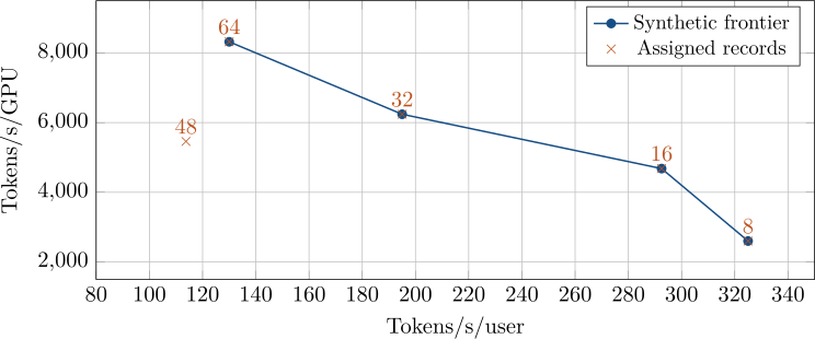
The released plotting script does something simpler: load_points retains the latest record at each scanned request count and checks a set of fixed configuration fields. Then line 150 plots all selected points in scan order. It does not calculate non-dominance or combine repeated runs statistically. A curve called “Pareto” still needs its points and assumptions examined [85].

11.6.2 The two meanings of acceptance

Chapter 2 established how to turn step rate into useful output. The decode plot makes that conversion explicit:

66xs = [p["decode_avg_sps"] * tau for p in points]
67ys = [p["decode_avg_sps"] * p["decode_num_requests"] * tau / p["cp"] for p in points]
68return xs, ys, [f"{p['decode_num_requests']:,}" for p in points]

Here $R=\mathtt{\text{decode\_num\_requests}}$ is per DP rank, and SPS is the measured decode steps per second, decode_avg_sps. The horizontal rate is $x=\mathrm{SPS}\tau$; the vertical rate is $y=\mathrm{SPS}\mathit{R\tau }∕\mathrm{CP}$. For the published decode figure, EP and DP are both 64, context length is 131,072, and nextn=3 is fixed. Its subtitle supplies 75% acceptance and $\tau =3.25$. The script calculates $\tau =1+\mathtt{\text{nextn}}\times a$ at line 61 and rejects variable-length mode at line 60. The acceptance value is an input to the plot, not an acceptance measurement in these records [85].

There are two plausible meanings of $a$. If it means the mean number of accepted draft tokens divided by three, then $\tau =1+3a$ is precisely the intended conversion, ignoring end-of-request clipping. But if it means a conditional acceptance probability of 0.75 at each successive draft position, chapter 8’s accepted-prefix rule gives

The second and third positions count only when all preceding draft tokens were accepted. Equal conditional probabilities suffice for this product; the lab uses independent Bernoulli draws as a simple exact enumeration of that case. One main-model token is included per step, with no early EOS in this model.

Lab 25 uses rational arithmetic to enumerate all eight acceptance patterns. The conversion results and the separate approximate image reading are:

Mean accepted fraction 0.75: tau=3.250000
Conditional acceptance 0.75: tau=2.734375
Common axis shrink: 15.8654%
Published point, approximate: 246 / 3.25 = 75.69 steps/s
Implied throughput at R=64, CP=1: 15744 tokens/s/GPU
Checks: exact prefix expectation and common-scale frontier passed

The ratio $2.734375∕3.25=175∕208$ shrinks both axes by about 15.9%. It preserves their relative order and which points are dominated if the same factor applies everywhere. If acceptance changes with workload or configuration, point-specific factors can change the frontier itself. The subtitle’s phrase “per-token acceptance” does not settle the definition, so this calculation identifies an assumption to check rather than proving that the figure is wrong.

11.6.3 Recover a step rate; specify the missing measurement

The published 64-request point is approximately 246 tokens/s/user, read from the image rather than a raw record. Under the figure’s $\tau =3.25$,

using CP=1. That agrees with the plotted point near 15,750. It is not the throughput of the entire 64-GPU instance. The image hash and fixed revision are recorded separately in the source manifest; the reading remains approximate.

Neither decode axis is a latency percentile. The reciprocal of user speed is an amortised time per output token; speculative steps can publish several tokens together. It does not reveal the gaps between bursts, queueing, or time to first token. The prefill figure uses mean measured step duration on its horizontal axis, which also omits a request’s earlier waits. Chapter 2’s request trace is the appropriate model for those quantities.

A measurement capable of changing the conclusion would record useful emitted tokens per request-step under the same model, prompt histories, sampling parameters and fixed draft length. It should count early termination and rejected drafts, then estimate $\tau$ at each concurrency instead of supplying one acceptance number. Keep raw records and token timestamps so that steady-state rates and end-to-end gaps remain distinguishable. First this checks the figure’s absolute scale; varying $\tau$ by point also tests its ordering.

The Wide-EP comparison needs a second control: repeat EP8 and EP64 on matched hardware and workload definitions, recording topology, model and dependency revisions, expert redundancy and the actual acceptance factor. Compare their frontiers at the same per-user target and per-GPU denominator, not merely at the same total request count. A different mapping from step rate to useful output could change the observed advantage. So could service queueing absent from the offline benchmark. This is a proposed measurement, not a result of our synthetic records.

11.7 Experiments to try next

1. In lab 23, use one decode worker instead of two. Predict which prefill saving survives in final completion time, then run your change. Identify the queue that absorbs the saved time.
2. Extend the local-cache case with a choice to recompute on the idle worker. Which hit lengths make affinity preferable under the assigned costs? State whether your objective is first completion, last completion or mean wait.
3. For a 902-token prompt, explain the different meanings of 768, 640 and 134 in lab 24. How many positions rebuild SWA when it is missing? Which block KV can still be reused? Why does this not resolve the 140-row keep setting?
4. A capacity estimate uses the fraction of requests with any cache hit as $h$. Construct two workloads with that same fraction but different uncached-token demand. Which measurement must replace it?
5. Change acceptance for just one synthetic operating point in lab 25. Can the set of non-dominated points change? Give the counts needed to measure that point’s $\tau$, including your treatment of completed requests.
6. Choose a service claim from Table 11.1. Locate the code, public project or Q&A passage that supports it, and name one observation needed to test its production behaviour.

11.8 One request, end to end

Follow request A with a 300-token prompt through the released offline path. Use a NORMAL engine, CP=1, ZOS enabled and fixed verification with nextn=5. Leave chunked prefill, YOCO truncation and structured output off. Assume enough free memory, no prefix hit or preemption, and an output limit that does not interrupt the steps below. Experts occupy the configured EP group; other requests keep decode calls running after A finishes. The lengths and acceptance outcome below are assigned to illustrate the inspected branches, not recorded engine output.

11.8.1 Admit the prompt and create the first output

LLM.generate admits A as a persistent Sequence in the waiting queue. When the scheduler selects its prompt, A receives three paged blocks, $\lceil 300∕128\rceil =3$, and a state slot. The block table locates compressed KV and index rows; the slot holds SWA and live compression state. No other request owns these allocations in this case (chapters 1, 4 and 5).

The worker sends the 300 prompt positions through embeddings and the model layers. Attention writes and reads the layer’s cache views; MoE sends each position’s expert work to the selected slots and returns the weighted results (chapters 3 and 7). Sampling uses the last prompt position’s representation to choose A’s first output. Prompt post-processing happens in the same worker call. The processed count is now 300, while token history has length 301. The output at position 300 still needs to become a model input.

11.8.2 Follow one six-position decode step

After further decode work, choose a step $N$ whose inputs begin at position 320 and include five available drafts. During call $N$, the host processes $N-1$: A’s committed count becomes 320 and its history length 321. Forward $N$ is already queued. Its six queries occupy positions 320–325, with key length 326. For example, position 320 lies in A’s third logical block at token-position offset 64; the block table supplies the physical block ID.

Assume verification accepts the first two drafts and rejects the third. The accepted prefix and its replacement contribute three output tokens. The six evaluated positions therefore advance the committed count by three, not six. The last output remains unprocessed:

Before that last update, scheduling $N+1$ sees 320 committed positions, six in flight and six new queries: an upper-bound key length of 332. On the device, the previous accepted count removes $5-2=3$, giving 329. The new queries actually cover positions 323–328. Their main input and drafts come from step $N$’s device output via the request remap, even though the host does not yet know them (chapters 6 and 8). The three blocks still suffice. Discarded draft bytes may remain in storage; counts and visibility decide which rows can be read (chapter 4).

Only after queuing forward $N+1$ does the worker wait for sample_end_evt(N) and post-process those three outputs. The entrypoint clones the returned pooled records while their addresses remain valid. Counting the six queries as six useful outputs would double this step’s progress; timing submission alone would miss the wait and publication boundary (chapters 1 and 2).

11.8.3 Finish, then change the boundary

Suppose a later step $M$ produces EOS. Call $M+1$ has already queued A’s extra forward before post-processing marks it finished. In call $M+2$, scheduling removes A; post-processing waits for the obsolete $M+1$ work and skips its output; pre_sampler_sync then releases A’s remaining storage. Other requests keep these decode calls consecutive, as assumed in chapter 6’s trace. At the eventual end of the whole generation loop, the final flush drains the remaining in-flight result. Request completion, output collection and storage release are distinct events.

Two changes connect this trace to the remaining chapters. Enabling compact prefill would introduce chapter 9’s full-source and retained-query layouts; agreement with mask would still not prove agreement with this untruncated baseline. Moving A to a disaggregated service would introduce prefix matching, PE selection and a PE-to-CE state handoff. The CE needs the live state extent, including the dropped region; the released layout helper does not implement that transport. These are changes to the case, not hidden steps in its offline execution.

Finally, choose the comparator before testing either change. Chapter 10’s golden trajectory can hold A’s tokens fixed for a numerical comparison; independently sampled outputs answer a different question. This single request now gives us both a route through the code and a way to investigate it: name the owner, locate the processed boundary, identify the completion condition, and state which observable a proposed change must preserve.