CHAPTER 07
Put experts on several devices
Chapter 3 placed attention and a feed-forward transformation inside each model layer. We now open that second part. DeepSeek’s V4 models use many networks called experts in their MoE layers. For every token, a gate scores the experts and chooses a few. Each token therefore uses only part of the layer’s weights, but different tokens use different parts. When the experts are spread over many devices, tokens must travel to the experts they chose, and the results must travel back.
The question
How does DeepInfer send each token’s expert work to the devices that hold those experts and bring the results back? Why can one busy device limit the benefit, and how does the engine move experts to reduce that imbalance?
7.1 Dispatch, compute and return
A layer built this way is a mixture of experts (MoE). The gate gives each token a short list of chosen experts and a weight for each. The layer’s output is the weighted sum of the chosen experts’ outputs. DeepSeek’s design also has a shared expert that every token uses, without being chosen [28].
python3 labs/15_dispatch.py
The experiment gives four experts, A to D, simple integer formulas, and the shared expert the formula . Two devices, called ranks, each own three tokens. Each expert occupies a slot on one rank. The routing weights are fractions, so the distributed result can be compared exactly with direct evaluation.
1. one expert per token: slots=['A', 'B', 'C', 'D'], top-1
  assignments per rank=[5, 1], busiest=5, sent to another rank=4
  per slot: 0:A=4, 1:B=1, 3:D=1
2. two weighted experts: slots=['A', 'B', 'C', 'D'], top-2
  assignments per rank=[8, 4], busiest=8, sent to another rank=6
  per slot: 0:A=5, 1:B=3, 2:C=2, 3:D=2
3. same experts, other placement: slots=['A', 'C', 'B', 'D'], top-2
  assignments per rank=[7, 5], busiest=7, sent to another rank=5
  per slot: 0:A=5, 1:C=2, 2:B=3, 3:D=2
4. replicas of A and B: slots=['A', 'B', 'C', 'D', 'A', 'B'], top-2
  assignments per rank=[6, 6], busiest=6, sent to another rank=4
  per slot: 0:A=2, 1:B=2, 2:C=2, 3:D=2, 4:A=3, 5:B=1
token results: (0, 0)=41/2, (0, 1)=21, (0, 2)=65/3, (1, 0)=107/3, (1, 1)=11, (1, 2)=124/5
The first run gives each token one expert. Dispatch sends each token’s value to the rank holding its expert. The receiving rank computes the result, and combine returns it to the token’s own rank. A token must carry its identity on the journey, or its result could not be put back in the right place. Four of six tokens chose A, so rank 0, which holds A and B, receives five of the six assignments.
The second run gives each token two experts with weights. A token now creates two assignments, possibly on different ranks. Each result is multiplied by its weight before it returns; the origin adds the shared expert’s output, computed locally, and the returned contributions. The script checks every token’s result against direct evaluation. Rank 0 receives 8 assignments and rank 1 only 4.
The third run moves B and C between ranks. Every token result is unchanged; only the work per rank and the number of assignments crossing ranks change. That is the freedom a placement policy uses.
The fourth run adds two slots, holding a second copy of A and of B. We now distinguish a logical expert, the function the gate chooses, from a physical expert, a copy of its weights in one slot. A copy is called a replica. A replica adds another place to compute A; it does not add an expert to any token’s choice. The lab picks a replica with DeepInfer’s rule, shown in the next section. Rank 0 and rank 1 now receive six assignments each, and the results are still unchanged.
The dispatch loop keeps the origin rank and token index with each assignment. replicas
maps an expert to its slots; integer division finds a slot’s owner:
per_rank = len(slots) // 2
replicas = {e: [s for s, name in enumerate(slots) if name == e] for e in EXPERTS}
inbox, sent = {0: [], 1: []}, 0
for token in TOKENS: # dispatch: each selection goes to one physical slot
rank, index, x, picks = token
norm = sum(w for _, w in picks[:top_k])
for expert, weight in picks[:top_k]:
copies = replicas[expert]
slot = copies[(rank + index * 23333) % len(copies)]
owner = slot // per_rank
inbox[owner].append(((rank, index), slot, x, weight / norm))
sent += owner != rank
Each owner computes its contributions. The same token key groups them on return, and
direct supplies a reference without dispatch:
partial = {} # compute on the owner; the weight is applied before return
for owner, items in inbox.items():
for key, slot, x, weight in items:
partial.setdefault(key, []).append(weight * EXPERTS[slots[slot]](x))
combined = {(r, i): shared(x) + sum(partial[(r, i)]) for r, i, x, _ in TOKENS}
expected = {(r, i): direct((r, i, x, p), top_k) for r, i, x, p in TOKENS}
The exact check proves that the teaching model routes and recombines correctly. It does not establish that DeepInfer’s floating-point kernels give bitwise-equal results for different placements; a different summation order can change the last bits.
7.2 Follow DeepInfer’s execution path
DeepseekMoE in v4_modules/mlp.py executes the layer; the neighbouring moe.py defines the
parameter containers it receives. Its constructor fixes the slot arithmetic (lines 196–202): the
number of physical experts is the number of routed logical experts plus the extra replica slots,
and each rank of the expert-parallel (EP) group holds an equal share. An assertion requires the
total to divide evenly [47].
The execution crosses several repositories, all within DeepSeek’s library stack. DeepGEMM, DeepEP and TileKernels supply kernels and communication; DeepInfer connects them to the model and the request loop. The boundary is concrete:
Boundary | Division of responsibility |
Replica selection | DeepInfer supplies logical-to-physical maps and replica counts; the DeepGEMM or TileKernels gate chooses a physical copy. |
Dispatch and combine | DeepInfer calls DeepEP’s |
Expert computation | DeepInfer selects the explicit or fused path and connects the shared contribution; DeepGEMM and TileKernels perform the kernel work. |
Load balancing | The statistics window, policy call, weight shuffle and mapping updates are implemented in this repository. |
The inspected calls and pinned dependencies establish these boundaries [47, 48, 55]. The model determines the routed expert functions and their selections. Extra physical copies are a deployment choice for serving uneven routed work, rather than additional logical experts required by the model.
7.2.1 From a token’s choice to a slot
The forward method has two paths. Begin with the explicit one:
if self.use_mega_moe:
return self.mega_moe_forward(hidden_states, hidden_states_bf16, input_metadata)
topk_idx, topk_weights = self.gate_forward(hidden_states_bf16, input_metadata)
try:
# Dispatch
event_overlap = self.dispatch(
hidden_states,
topk_idx,
topk_weights,
input_metadata,
None,
)
moe_in_hidden, _dispatched_topk_idx, dispatched_topk_weights, handle = event_overlap.current_stream_wait()
The gate returns, for each token, the chosen experts and their weights. Those indices are already physical slots. The gate receives the load balancer’s maps:
to_physical_map=eplb_layer.logical_to_physical_map,
logical_count=eplb_layer.logical_count,
scoring_func=self.scoring_func,
out=out,
)
if self.use_mega_gate:
topk_idx, topk_weights = deep_gemm.bf16_mega_gate(hidden_states, self.gate.weight, **gate_kwargs)
else:
topk_idx, topk_weights = moe_topk_gate(self.gate(hidden_states), **gate_kwargs)
to_physical_map lists the slots holding each logical expert, and logical_count
says how many there are. On GPUs the gate runs in DeepGEMM’s bf16_mega_gate;
otherwise it uses the TileKernels gate. Both are DeepSeek libraries maintained in separate
repositories. At DeepInfer’s pinned submodule commit, DeepGEMM chooses a replica by
where token is the token’s index in its own rank’s batch. The source comment says the
purpose: spread one logical expert’s tokens over its replicas, differently on every rank. The
TileKernels version required by DeepInfer uses the same rule [52, 53].
The rule does not look at current load. It spreads tokens by their index, so replicas share work only approximately. In lab 15, A’s five assignments split two and three. The placement policy later in this chapter assumes an equal split; that assumption is an estimate.
Follow token
in the lab’s fourth run. Its value is 5 and its logical choices are A and C, each with weight
. The layout is ABC/DAB, so
A’s slots are and C’s only slot is
2. For A, the replica rule gives :
the second copy, slot 4 on rank 1. For C it gives zero: slot 2 on rank 0. The equivalent row of topk_idx is
therefore , paired
with topk_weights .
7.2.2 Through the experts and back
dispatch hands the hidden states, slot indices and weights to DeepEP’s communication buffer
[47]. Like the asynchronous work in chapter 6, the transfer runs on its own schedule.
current_stream_wait makes the compute stream wait for its event before using what arrived.
The results are the rows received by this rank, their weights and a handle. The handle carries the
bookkeeping needed later: how many received rows belong to each local expert, used by the
expert computation (line 596), and the routing information needed to send results
home.
For our token, dispatch sends one row to rank 1’s local slot 1 (global slot 4) and one to rank
0’s local slot 2. The received weights follow those rows into routed_experts_forward; the
handle’s psum_num_recv_tokens_per_expert describes their grouping by local expert.
DeepInfer’s rows are hidden-state vectors; the lab uses the scalar 5 so that we can calculate the
contributions by hand.
Where do the weights take effect? Not in combine. Inside the expert computation, the activation step receives them:
down_in_hidden = swiglu_forward_and_per_token_cast(
gate_up_proj_out,
**_get_swiglu_kwargs(self.use_fp8_act),
psum_num_tokens_per_expert=psum_num_recv_tokens_per_expert,
topk_weights=topk_weights,
clamp_value=self.swiglu_clamp_value,
)
This matches the lab, which multiplies each result by its weight before return. The name
combine could suggest that the weighted sum happens there; the code shows that the rows are
already weighted when they leave the experts.
Return and the shared expert follow:
# Combine
combine_pre_evt = self.ep_buffer.capture()
with limit_num_sms(envs.DEEPINFER_USERBUFFER_COMM_SMS, enabled=PLATFORM.is_gpu):
shared_out = self.shared_forward(hidden_states)
event_overlap = self.combine(
moe_out_hidden,
shared_out,
handle,
combine_pre_evt,
)
moe_combined_hidden, _combined_topk_weights = event_overlap.current_stream_wait()
The shared expert runs on the token’s own rank. limit_num_sms lowers the number of
streaming multiprocessors that its kernels may use by the number set aside for communication, so
the transfers keep their share of the device (parallel_utils/userbuffer.py, lines 40–51).
combine passes its output as bias (line 505): the shared contribution is added when the routed
results arrive. A token’s final row is therefore the shared output plus its weighted routed results,
as in the lab [47].
In the scalar trace, A returns
from rank 1 and C contributes
on rank 0. The dispatch handle lets combine return the remote contribution to the original row on rank 0. The
shared contribution is ,
supplied as bias in the explicit engine path. The final value is
, the lab’s
result for .
7.2.3 The fused path
The explicit stages are a readable account of the data movement, but they are not the only path.
Lines 184–188 require the whole EP group to lie within one NVLink domain, a set of
devices joined by a fast direct interconnect. They also require either a GPU platform
or FP8 activations with FP4 weights, and a supported matrix-multiplication format.
When these conditions hold, forward returns early through mega_moe_forward (lines
528–563).
That method still calls gate_forward, writing the choices into a symmetric buffer
shared across the group. A single DeepGEMM call then receives the buffer, both expert
weight matrices, the shared-expert weights when they are fused, and the load counter
discussed below (line 555). The routing, expert work, shared work and load counting
are all present; they are no longer separate Python stages. The README reports its
decode benchmarks on 64 GPUs within one scale-up domain, the setting in which
this condition can hold, but the book has not established which path those runs took
[47, 1].
7.3 Why widen the expert group?
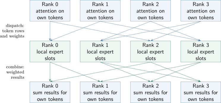
Figure 7.1 shows the arrangement the deployment Q&A describes for V4.1 decode. Attention runs with data parallelism (DP): each rank processes its own requests. The MoE stage runs with expert parallelism over the same ranks, with the DP size equal to the EP size. The Q&A reports decode groups of EP64 to EP128, calls this Wide-EP, and says that it substantially reduces per-step memory traffic in the expert part [2]. The released code supports other group sizes; these numbers are a reported production setting.
Chapter 2’s cost model explains the attraction. Take an illustrative layer with routed experts, each token choosing , and tokens per rank. These are teaching numbers, not V4.1’s configuration. With ranks and no replicas:
| Ranks | Experts per rank | Mean assignments per expert |
| 8 | 32 | 8 |
| 64 | 4 | 64 |
Holding the per-rank batch fixed, the wider group gives each rank fewer expert weight matrices to read per layer, and each matrix serves more tokens on average. In chapter 2’s terms, the expert computation moves towards higher arithmetic intensity. The comparison assumes every expert receives some tokens, the same model and the same hardware.
Two costs limit the gain. Each rank still sends assignments and receives their results, whatever the group size, and in a wider group a larger share of them leave the rank. The step must also wait for the slowest rank. Lab 15’s second run had 8 assignments on one rank and 4 on the other. Those counts identify the busiest rank in the lab; it has no duration model. Kernel efficiency and communication also affect the time, so the counts do not establish step latency.
7.4 Use history to choose a placement
The engine reduces imbalance with expert-parallel load balancing (EPLB): it observes which experts were busy and periodically changes which slots hold which experts. Figure 7.2 shows the cycle.
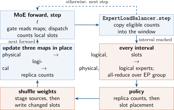
step records load statistics and clears the counter before the next
forward pass [47, 48, 49, 50].
7.4.1 Counting work
The counter appears in the MoE calls themselves: explicit dispatch passes the layer’s
expert_count as cumulative_local_expert_recv_stats (line 474), and the fused call passes
the same tensor (line 555). It has one entry per local physical slot and layer.
After sampling, DeepseekForCausalLM calls ExpertLoadBalancer.step (deepseek.py, lines
402–404). That method updates the rearrangement history when enabled, records load
statistics and finally zeroes the counter. The rearrangement history is a ring of recent
steps, the window. Every interval of eligible steps, it triggers _rearrange_experts
[48].
The policy needs counts per logical expert across the whole group, not per local slot.
First, _rearrange_experts selects this rank’s mapping and allocates space for logical
counts:
window_size, num_moe_layers, num_local_physical_experts = self._expert_count_window.shape
num_physical_experts = self.physical_to_logical_map.shape[1]
num_logical_experts = self.logical_count.shape[1]
local_physical_to_logical_map = self.physical_to_logical_map[
:,
ep_group.rank() * num_local_physical_experts : (ep_group.rank() + 1) * num_local_physical_experts,
]
logical_expert_token_counts = torch.zeros(
window_size,
num_moe_layers,
num_logical_experts,
dtype=torch.int,
device=local_physical_to_logical_map.device,
)
Next, scatter_add_ adds each local slot’s count to the logical expert that slot held.
The all-reduce sums over ranks, so replicas on different ranks contribute to one logical
total:
logical_expert_token_counts.scatter_add_(
-1,
local_physical_to_logical_map.to(torch.int64).expand_as(self._expert_count_window),
self._expert_count_window,
)
dist.all_reduce(logical_expert_token_counts, group=ep_group)
next_physical_to_logical_map, next_logical_to_physical_map, next_logical_count = rebalance_experts_global(
logical_expert_token_counts,
num_physical_experts,
num_local_physical_experts,
)
The window keeps one row per step; it does not add the steps together. The policy uses that structure.
7.4.2 Why keep the steps separate?
python3 labs/16_placement.py
This experiment requires PyTorch, but no GPU. It loads an unmodified copy of DeepInfer’s
policy.py, checked against the source manifest, and calls rebalance_experts_global directly.
It imports nothing else from the engine. The saved output records the PyTorch version in
results/provenance.json.
History by step: [[10, 10, 0, 0], [0, 0, 10, 10]]
  candidate AB/CD: score=40
  candidate AC/BD: score=20
  policy AC/BD: score=20

Skewed history by step: [[30, 6, 4, 0], [20, 10, 0, 6], [40, 2, 6, 2]]
  initial ABC/DAB: score=70.00
  policy AAD/ABC: score=68.00
  physical->logical: ['A', 'A', 'D', 'A', 'B', 'C']
  logical->physical: {'A': [0, 3, 1], 'B': [4], 'C': [5], 'D': [2]}
  replicas: {'A': 3, 'B': 1, 'C': 1, 'D': 1}
The first history has four experts, two ranks and two slots per rank. In step 1 only A and B are busy; in step 2 only C and D. Over both steps every expert has 10 tokens, so both placements give each rank a total of 20. The steps tell a different story. With AB/CD, rank 0 does all the work in step 1 and rank 1 all of it in step 2: the busiest rank carries 20 in each step, 40 in total. With AC/BD, each rank carries 10 in each step, and the policy chooses AC/BD. A policy that saw only the totals could not tell the two placements apart. The policy’s score is the sum over steps of the busiest rank’s estimated load:
The lab loads the checked file directly, bypassing the package initialisers:
def load_policy():
spec = importlib.util.spec_from_file_location("eplb_policy", POLICY)
assert spec is not None and spec.loader is not None
module = importlib.util.module_from_spec(spec)
spec.loader.exec_module(module)
return module
Its place function adds a one-layer dimension to the history, calls the real policy and checks
the returned maps and replica counts:
def place(policy, history, num_physical, per_rank):
tokens = torch.tensor([[step] for step in history], dtype=torch.int) # [steps, layers=1, experts]
p2l, l2p, count = policy.rebalance_experts_global(tokens, num_physical, per_rank)
slots, l2p, count = p2l[0].tolist(), l2p[0].tolist(), count[0].tolist()
for expert, physical in enumerate(l2p): # check both maps and the replica counts
valid = [p for p in physical if p >= 0]
assert len(valid) == count[expert] == slots.count(expert)
assert all(slots[p] == expert for p in valid)
assert len(slots) == num_physical and sum(count) == num_physical
return slots, l2p, count
7.4.3 Two decisions: replicas, then places
rebalance_experts_global first decides how many copies each logical expert gets. One extra
slot at a time, it asks which expert’s copy would most reduce the sum over steps of the largest
per-copy load:
score = tokens_per_expert_all_diff / logical_count # NOTE: Values in score must be different from each other
score_added = tokens_per_expert / (logical_count + 1)
values, indices = score.max(-1, keepdim=True)
values = values.expand_as(score).contiguous()
score.scatter_(-1, indices, score_added.gather(-1, indices))
values.scatter_(-1, indices, score.max(-1, keepdim=True).values)
score is each expert’s load per copy in each step. score_added is what it would be
with one more copy. Giving a copy to the current busiest expert lowers the maximum;
giving it to anyone else leaves the maximum unchanged. After these lines, values
holds, for each candidate, the step’s largest per-copy load if that candidate received the
copy. Summing over steps and taking the smallest picks the replica (line 117). Line
109 adds a tiny amount per expert so that equal loads still have a single maximum
[49].
In the lab’s skewed history, A carries 30, 20 and 40 tokens in the three steps, far more than any other expert. Both extra slots go to A, giving it three copies.
The second decision places the six copies on two ranks of three slots each. The
helper that does this, _batch_greedy_indices, takes the copies in descending order of
their total per-copy load over the window (lines 31–35). For each copy it computes, for
every rank, the score that would result from placing it there (lines 58–60): each step’s
busiest-rank load after the addition, summed over steps. It then commits the best
rank:
rank = scores.argmin(dim=-1)
occupied = occupancy[layers, rank]
indices[layers, rank * capacity + occupied] = physical_order[:, job_index]
occupancy[layers, rank] = occupied + 1
updated = loads[layers, rank] + vector
loads[layers, rank] = updated
torch.maximum(peaks, updated, out=peaks)
Full ranks were excluded on line 62, and argmin breaks ties towards the lower rank. The result
in the lab is AAD/ABC, with an estimated score of 68. The starting layout, ABC/DAB, which
gives the two extra slots to A and B, scores 70. The lab checks that both maps agree: every slot
listed for an expert holds that expert, and each expert’s replica count equals its number of
slots.
These scores are estimates in the policy’s own model. The policy divides an expert’s load equally among its copies, whereas the gate’s index rule splits them approximately. The algorithm is greedy, so it does not guarantee the best placement. The score leaves out communication, kernel efficiency and the cost of moving weights. A difference between 70 and 68, or between 40 and 20, is not a measured speed-up.
7.4.4 Compare two DeepSeek placement policies
DeepSeek also published a standalone EPLB implementation. At the fixed commit d52c72d, it
already separates logical experts from physical replicas, allocates redundant copies and
packs them into equal-capacity device groups. Its entry point returns the same three
kinds of map/count tensors. Its README leaves load prediction to the caller and
suggests a moving average of historical statistics [54]. The useful comparison is therefore
how the two policies represent and use load, not whether replication first appears in
DeepInfer.
Decision | Standalone
EPLB
at
| DeepInfer
at
|
Load input | One scalar per layer and logical expert. | One count per step, layer and logical expert. |
Next replica | Copy the expert with the largest scalar load per existing replica. | Score each candidate by the sum of per-step maximum per-copy loads after adding it. |
Placement | Sort scalar copy loads, then choose the least-loaded pack with space. | Sort total copy loads, then score candidate ranks using per-step maximum rank loads. |
Topology | Entry point selects hierarchical group/node packing or a global fallback. | The inspected global policy takes physical and per-rank slot counts, without group/node parameters. |
In the standalone code, replicate_experts chooses copies and balanced_packing places them. The
entry point is rebalance_experts. Compare these with the two DeepInfer functions just read
[54, 49].
The input difference can change a decision. Consider two experts with loads in one step and in the next, and one spare slot. If the caller supplies totals to the scalar policy, it copies A. Keeping both steps, a copy of A gives per-step maxima 5 and 18, summing to 23; a copy of B gives 10 and 10, summing to 20. DeepInfer’s replica score therefore chooses B. The third case in lab 16 calls DeepInfer’s policy with this history, three physical slots and one slot per rank. It checks the returned maps and asserts the replica counts:
Replica-choice history by step: [[10, 0], [10, 18]]
  replicas: A=1, B=2
These are calculated loads, not timings. The standalone policy is compared by source inspection; this lab runs only DeepInfer’s policy. The chapter’s AB/CD example shows the same information loss at the placement stage.
This fixed-version comparison establishes implementation differences. It does not identify a direct code lineage between the repositories or show that one policy is always better. DeepInfer’s runtime contribution, which we follow next, is to collect the history and make the chosen placement take effect between model steps.
7.5 Make the new placement take effect
7.5.1 The slot budget is fixed
Extra slots cost memory: each holds a full copy of one expert’s weights in every MoE
layer. The number is fixed when the model is built. The loader reads a requested
minimum from DEEPINFER_OVERRIDE_NUM_EXTRA_EXPERTS, which defaults to zero, and
resolve_num_extra_experts rounds it up so that the total divides evenly among EP ranks
(model_loader.py, lines 83–107; eplb/__init__.py, lines 21–28). The example setup requests at
least 32 (examples/_config.py, lines 77–79). As an illustration, 256 routed experts
plus 32 requested extras make 288 slots; at EP64 the engine adds 32 more so that
. The
Q&A reports, for decode, one extra slot per GPU before rounding [51, 48, 17, 2].
A later policy call does not add slots. It only chooses which logical experts occupy them. Comparing configurations with different slot budgets must therefore charge the extra weight memory: device memory that chapter 4’s block pool could otherwise use.
7.5.2 Move weights, then switch the maps
After the policy returns, _rearrange_experts moves weights and installs the new
maps:
if self._intranode_shuffle:
expert_model_parallel_shuffle_inplace_intranode(
self._ipc_weight_buffers,
self.physical_to_logical_map,
self._expert_weights,
next_physical_to_logical_map,
ep_group,
)
else:
expert_model_parallel_shuffle_inplace(
self.physical_to_logical_map,
self._expert_weights,
next_physical_to_logical_map,
ep_group,
)
self.physical_to_logical_map.copy_(next_physical_to_logical_map)
self.logical_to_physical_map.copy_(next_logical_to_physical_map)
self.logical_count.copy_(next_logical_count)
The three tensors are updated in place. The per-layer state that the gate receives is a view of those same tensors (lines 346–376), so the next forward pass reads the new mapping without any other hand-over. The weights must already be in their new slots when that happens, which is why the shuffle comes first. The rank-0 metrics path synchronises the device around the operation and logs its elapsed time (lines 226–228 and 280–288) [48].
Moving weights has its own hazard. Suppose slot 2 should receive the expert that slot 5 holds,
while slot 5 should receive slot 2’s expert. Copying one directly into the other would destroy a
source that is still needed. The general point-to-point shuffle avoids that by staging. Copies
within a rank and transfers from other ranks both write into separate receive buffers first
(shuffle.py, lines 107–138). Only after every transfer has completed does it write the changed
slots:
recv_slot = dict(experts_to_recv)
for i in range(num_local):
if origin_local[i] == current_local[i]:
continue
src = i if received[i] else recv_slot[current_local[i]]
for weight, buf in zip(weights, recv_buffers, strict=True):
weight[i].copy_(buf[src])
Unchanged slots are skipped. A changed slot takes its new weights either from its own staged copy or from the buffer that received that expert from another rank. When the whole group lies within one NVLink domain, the intranode path instead copies each rank’s weights into a shared mirror, one layer at a time. Two barriers bracket the mirror refresh; their comments say, in the author’s translation, “wait for every rank to finish reading the previous layer’s mirror” and “wait for every rank’s mirror to be ready” (lines 192–195). Reads then come from mirrors, or from a slot that has already received its new weights [50].
Apply the general shuffle to the lab’s actual transition, ABC/DAB to AAD/ABC. Global slot 2 on rank 0 must change from C to D. D currently lives in global slot 3, rank 1’s local slot 0. Rank 1 sends those weights into rank 0’s receive buffer at local index 2. Once the transfer completes, the final loop copies that buffer entry into rank 0’s weight slot 2. Meanwhile C must move from old slot 2 to rank 1’s slot 5. Staging both transfers preserves C before slot 2 is overwritten. Figure 7.3 shows these two transfers; the other changed slots use the same shuffle.

Only after the shuffle is queued does the engine queue the three
tensor updates. For this layer, physical_to_logical_map becomes
.
The valid entries in logical_to_physical_map are A:
, B:
, C:
, D:
, with
logical_count .
A’s list is in the order returned by the policy, not sorted slot order; the replica formula indexes
that list. These are the lab’s actual outputs.
On the next forward pass, consider token
, which
selects D in lab 15. D still has one replica, so its replica index is zero. The gate now reads
logical_to_physical_map[D,0] as 2 rather than 3. Dispatch therefore sends that assignment to
rank 0 rather than rank 1, and the destination slot now holds D’s weights. The logical
computation is unchanged; its location has changed.
7.5.3 When rearrangement runs
Rearrangement is off by default. DEEPINFER_EXPERT_REARRANGEMENT_STEP_INTERVAL defaults to
zero, and _update_rearrangement returns early in that case (environ.py, lines 115–117;
eplb/__init__.py, lines 147–148). For an EP group with more than one rank, step still calls
_update_load_balance_stats and clears expert_count (lines 131–138). Load statistics,
including their periodic collective, remain active when rearrangement is off; this is the statistics
flush discussed in chapter 2. When it is enabled, the window must lie between one step and the
interval (lines 106–111), and the first rearrangement comes after a quarter of the interval,
to correct start-up imbalance sooner (lines 121–123). A normal engine leaves prefill
steps out of the window unless a separate setting asks for a rearrangement straight
after prefill (lines 83–84 and 149–159). The example setup uses a three-step window
and, when EPLB is enabled, a 30-step interval (examples/_config.py, lines 80–83)
[30, 48, 17].
The deployment Q&A reports very different production settings: a 100-step window and a 1,000-step interval for prefill, and 1,000 and 10,000 for decode. It reports a ratio of slowest to mean rank load of 1.074 and 1.045 for two prefill configurations and 1.090 for decode [2]. Those are DeepSeek’s reported measurements; this book has not reproduced them.
Both settings reflect a trade. A placement is chosen from the past, so it lags a workload that changes. Moving weights takes time on every rank. As a teaching model only: if a rearrangement costs seconds and saves seconds per step for the next steps, it pays when . Long intervals bet that expert popularity changes slowly. The rank-0 log already records rearrangement time, which supplies an observation of . This book has not run the engine to obtain that value or measured the subsequent saving and how long it persists. Choosing needs those measurements.
We can now follow a token’s expert work from the gate to another rank and back, and follow the counts it leaves behind into a new placement. These choices affect the cost of a forward pass. The next chapter asks which draft positions are worth evaluating at that cost, allocating a verification budget across requests using predicted useful output and measured step times.
7.6 Experiments to try next
- In
labs/15_dispatch.py, give token the choices A and D. Predict the per-rank assignments in runs 2 and 4 before running the script. - Change the replica rule in the lab to always pick the first copy. Which rank becomes busiest in run 4? What does the index rule buy, and what can it not guarantee?
- In
labs/16_placement.py, add a third step in which only A and C are busy. Does the policy still choose AC/BD? Compute both scores by hand first. - Give the skewed history four slots per rank. How many replicas does each expert receive, and does the score improve? Relate the extra slots to weight memory.
- Using the teaching model , list the quantities you would need to measure to choose a rearrangement interval, and where in DeepInfer you would record each one.